2.1. The Ray Model for ARCs
Directional emission from ARCs enables measurements of optical modes in the far field. Directional emission has been studied extensively with various resonators geometries, including ellipse, half-circle-half-quadrupole (HCHQ), and even an egg shape resonator [
18,
22,
29,
30]. The boundary shape and degree of deformation have significant impact on the coupling and emission points as well as on the coupling efficiency to optical modes.
The mechanism for directional emission from a microcavity can be understood through a 2D chaotic billiard model. An ensemble of rays seeded into a microcavity with a given boundary and followed for a large number of internal reflections can be plotted in phase space, where each point identifies a reflection at the cavity boundary. The resulting map is known as a Poincare Surface of Section (PSOS) [
21,
32,
33]. These plots are the stroboscopic view of a chaotic billiard system, where sinχ, the sine of the incident angle of any given reflected ray is plotted versus Φ, the polar angle at which the ray is reflected at the cavity boundary. These ray tracing simulations, have been studied extensively in the literature, and the directional emission behavior suggested by the theory has been measured experimentally in quadrupole and half-quadrupole-half-circular (HQHC) shaped boundaries [
21,
23,
32,
34,
35]. By iteratively following the points in PSOS plots, indicating the successive reflection of rays, it can be shown that chaotic ray trajectories evolve in phase space along well defined paths called “unstable manifolds” [
32,
33,
36,
37]. Each point along the unstable manifold is defined by the coordinates (Φ, sinχ), and can represent the point of refractive escape if sinχ equals sinχ
c, the critical angle for internal reflection in a specific ARC. In other words, the unstable manifolds map the polar coordinates of refractive escape for a complete range of sinχ
c values. Ray diffusion along the path of unstable manifolds with resulting tangential emission is a good approximation for ARCs with small deformation. With small variation in sinχ for successive reflections, rays escape the cavity at angles very close to the critical angle and thus, as a result of Snell’s law, escape nearly tangent to the boundary [
32].
We examine the angles of refractive escape from 2D disk-shaped microcavities where the boundaries are defined by the quadrupole polar equation:
where ε is the degree of deformity ε = (R
a – R
b)/(R
a + R
b), R
a and R
b are the length of major and minor axis respectively. R
0 is the non-deformed radius, and
m is the number of poles in the boundary [
31,
38]. For the ray-tracing simulation in
Figure 1, sinχ
c was set as 0.68, to simulate a fused silica resonator,
i.e., SMF-28 glass of index n~1.47 in air. R
0 is arbitrary to the directional emission patterns and thus defined as 1, and ε was defined as 0.1, 0.05, and 0.025 for the 2-pole, 3-pole, and 4-pole ARCs respectively. As shown in
Figure 1, using this equation, the number of poles directly impacts the number of distinct emission points, and for these conditions, the unstable manifolds intersect sinχ
c at polar angles (Φ
emission) corresponding to the points of highest curvature along the resonator boundary. Thus rays exclusively escape from these points of highest curvature,
i.e., where the poles exist.
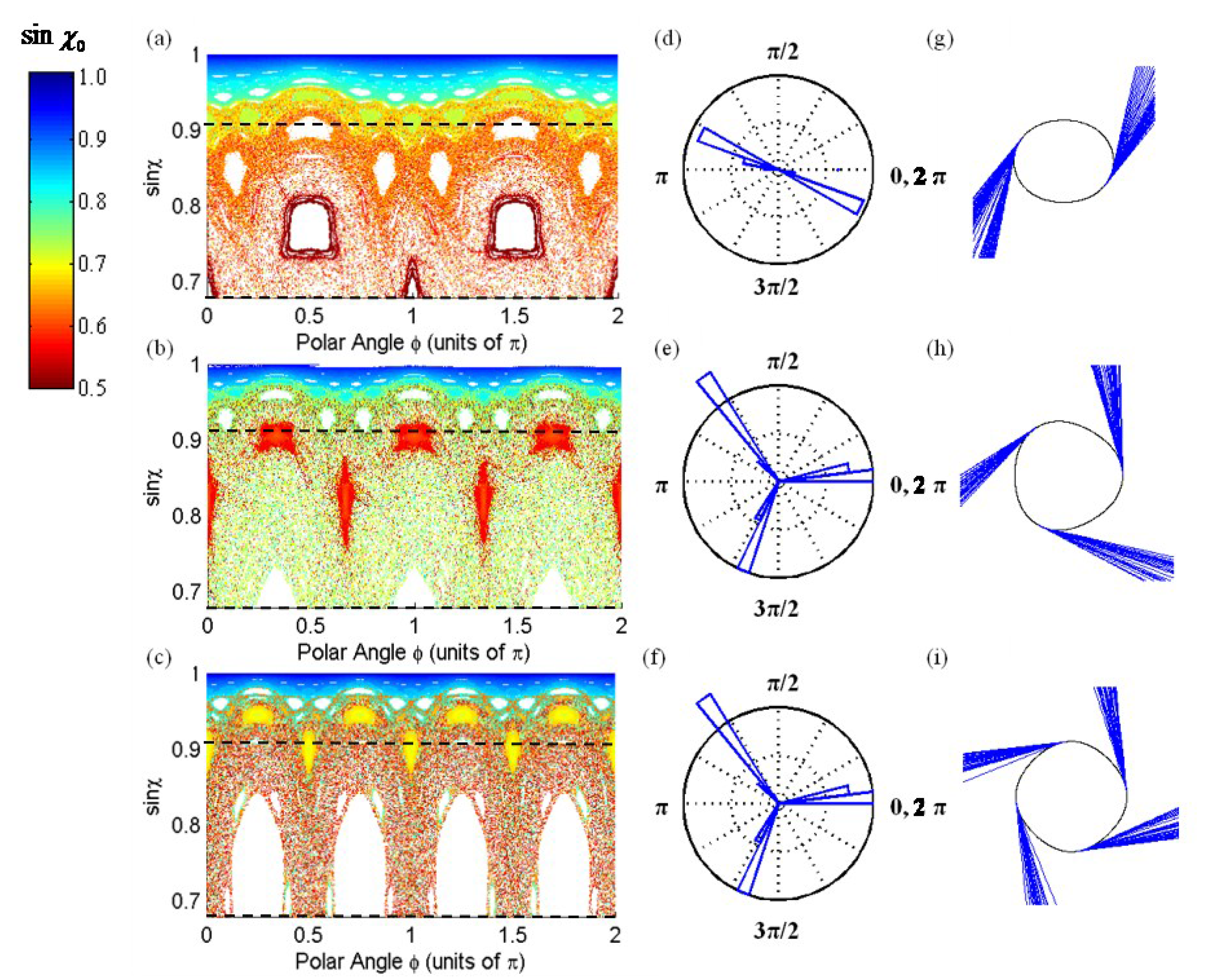
Figure 1.
(a–c) PSOS plots for two, three, and four-pole boundary shapes where the color of each point corresponds to the initial sinχ0 value of the injected ray. For this simulation 250 rays were seeded into the 2-D boundaries at π/2 with an initial linear angular spread from 45° to 90° and followed for 3000 reflections. The dotted lines at sinχ = 0.68 and sinχ = 0.91 indicate the sinχc for a SMF-28 (n~1.47) resonator in air and water respectively; (d–f) histogram plots of the polar angle at which rays escape refractively from the cavity in air (g–i) the corresponding ‘m-pole’ boundary shape with the exiting rays from the chaotic billiard simulation.
However, if the resonator is placed in a higher index environment such as water (n ~ 1.34), the sinχ
c value increases, which causes changes to the directional emission strength. This is due to the fact that fewer of the rays seeded at random sinχ values (and fixed coupling angle ϕ = π/2) at the onset of our PSOS calculation are trapped by total internal reflection and guided via chaotic trajectories to particular emission points. In other words, an ARC with a low sinχ
c value due to immersion in a lower index environment enables a greater number of randomly seeded rays to propagate via total internal reflection in the ray-tracing simulations. As illustrated in
Figure 1, the critical angle cut-off for SMF-28 in air (sinχ
c~0.68) enables a much larger region of the chaotic sea to exist within the resonator as opposed to the critical angle cut-off for SMF-28 in water (sinχ
c~0.91). For SMF-28 in air, a larger fraction of randomly seeded rays thus participate in the “chaotic sea” and are guided via the unstable manifolds to their directional emission points. As observed from our simulations, this results in stronger directional emission patterns when comparing the ARC in low index environments versus the ARC in higher index environments, and suggests more efficient free space coupling when comparing the former to the latter.
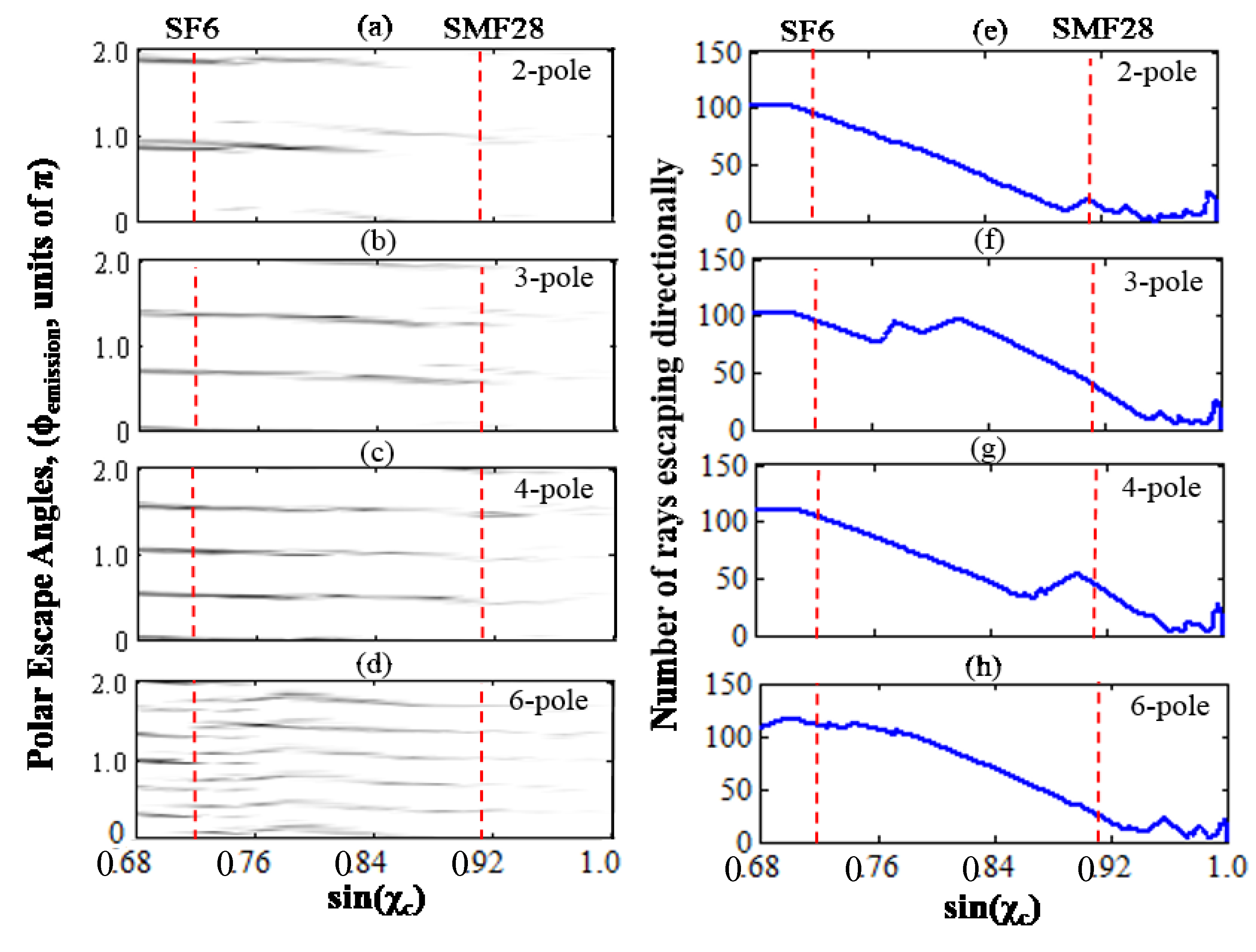
By further analyzing the results of the ray-tracing simulation, the number of rays which are trapped by total internal reflection and guided to directional emission points can be determined as a function of sinχ
c,
Figure 2.
Figure 2.
Further analysis of the ray-tracing simulation. (a–d) shows the polar escape angles (ϕemission) of the rays as a function of the critical angle parameter (sinχc). The gray value indicates the number density of the rays guided via chaotic trajectories to directional emission points; (e–h) shows the total number of rays esca** at directional emission points for a certain sin(χc) in the ray-tracing simulation of 250 randomly seeded rays (i.e., the integration of (a–d) along ϕ) The dotted red lines indicate the critical angles for SF6 glass in water (sinχc~0.72) and SMF-28 glass (sinχc~0.91) in water.
Therefore, the ray model seems to suggest that in order to maintain strong directional emission and thus, in reverse, efficient free-space coupling in higher index environments, the ARC resonator refractive index should be raised in order to decrease the sinχc value. In our simulations, this allows for more rays to be trapped in the chaotic sea by total internal reflection and guided to emission points. Specifically, for biodetection measurements, the SMF-28 silica resonators (n ~ 1.47) in water seems unfavorable, because the high sinχc value supports only a small fraction of seeded rays to be guided via total internal reflection to the directional emission points. Thus a higher index glass such as SF6 (n ~ 1.86) should be more suitable for practically achieving more efficient free-space coupling in aqueous environment. Furthermore, SF6 can provide cavities with a material limited Q factor of ~1.3 × 10⁷, and a laser source exhibiting minimal absorption losses in aqueous environment when operating at ~405 nm nominal wavelength, close to the absorption minimum of water, can be used to maintain high Q factors even after immersion in water.
2.2. Visualizing Directional Emission Patterns from ARCs
To test the trends predicted by our simulations, microspheres were fabricated by melting standard SMF-28 fibers (n ~ 1.47) as well as SF6 fibers (n ~ 1.86) into spherical shapes with diameters of 30–80 μm. Then, slight deformations were introduced to the spheres by a series of 10–20 ms pulses from a focused 30 W CO
2 laser operating at 20% of its duty cycle [
23]. Typically, to induce an effective deformation, resonators were pulsed two to three times on two opposite sides. Deformation parameters were then resolved with a 10× imaging system, and analyzed with Image
J. For this specific study, ARCs were fabricated with a deformation parameter of ε < 2%. However, because the deformation is small (ε < 2%), accurately defining a function describing the boundary shape of the ARC is very difficult with optical imaging alone. We therefore implement an approach based on fluorescence imaging to directly visualize the emitted light pattern of the ARC, identify the number of poles, and thus assign a theoretical boundary shape that can predict the observed emission properties.
Figure 3.
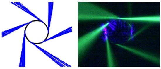
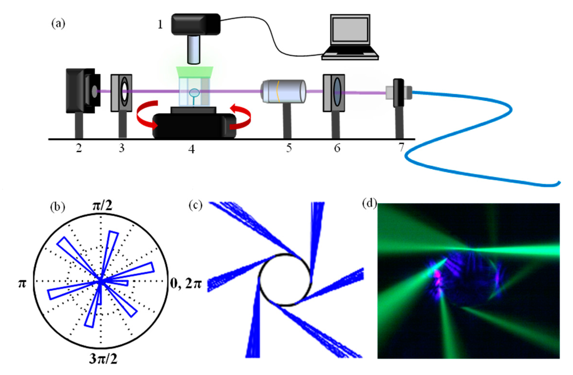
(a) Experimental set-up for visualizing directional emission of ARCs in aqueous solution: 1. Imaging system 2. Photodetector for measuring modes in the far field 3. Spatial filter for isolating far field emission pattern. 4. Rotation stage, with ARC and chamber with GFP in PBS buffer 5. The 10× objective is used for focusing the coupling beam 6. Quarter-wave plate for polarization control 7. Fiber collimator (b) Polar histogram of refractive escape for 6-pole boundary ARC from (c) simulation of refractive escape of rays injected into the ray-tracing simulation (ε = 0.01) (d) real color image of directional emission by GFP fluorescence imaging of 63 μm diameter ARC fabricated from SF6 fiber.
Figure 3.
(a) Experimental set-up for visualizing directional emission of ARCs in aqueous solution: 1. Imaging system 2. Photodetector for measuring modes in the far field 3. Spatial filter for isolating far field emission pattern. 4. Rotation stage, with ARC and chamber with GFP in PBS buffer 5. The 10× objective is used for focusing the coupling beam 6. Quarter-wave plate for polarization control 7. Fiber collimator (b) Polar histogram of refractive escape for 6-pole boundary ARC from (c) simulation of refractive escape of rays injected into the ray-tracing simulation (ε = 0.01) (d) real color image of directional emission by GFP fluorescence imaging of 63 μm diameter ARC fabricated from SF6 fiber.
For establishing fluorescence imaging of the emission pattern, ARCs were submerged in chambers of 10 µg/mL Green Fluorescent Protein (GFP) (Active
A. victoria GFP full length Protein ab84191) in a PBS buffer (pH 7.0). The beam waist of the 405 nm laser was brought just to the outside of the resonator boundary, and the resonator was rotated to the optimal coupling spot along the circumference. An imaging system directly above the resonator was then able to capture the ~509 nm fluorescent emission from the GFP, thereby spatially resolving the directional emission pattern as well as the incoming beam (
Figure 3).
We tested our hypothesis of maintaining directional emission in higher index environments through the use of higher index resonators made from SF6 fiber as compared to those made from SMF-28 fiber. Once free space mode coupling to our SF6 resonators was confirmed in air, see also next
Section 3, the GFP solution was injected into the chamber and the fluorescence signal was imaged.
Figure 3d is, to the best of our knowledge, the first direct, comprehensive experimental visualization of directional emission due to the chaotic nature of ray-dynamics. The observed emission pattern can be recreated with the ray-tracing simulation by implementing a boundary with six poles and deformation parameter (ε) of 0.01. For all the SF6 resonators fabricated, emission patterns with six or seven poles were observed by imaging. Consistent with the trends for coupling efficiency predicted by our PSOS plots, we only observe excitation of higher Q resonances (WGMs) with SF-6 ARCs in water, as we will show in the following, and report no observation of microcavity resonances of significant Q factors for free space coupling to SMF-28 ARCs after their immersion in an aqueous environment. This positive result for SF6 agrees with the hypothesis made in
Section 2.1, but the high number of poles in the boundary is surprising. Most literature up to date, which has not yet directly imaged the emission pattern, has only measured ARCs with either two or four emission directions in the far field theoretically defined by quadrupole or half-quadrupole-half-circle boundaries [
21,
35,
39,
40]. However, the observed 6‒7 pole emission was repeatable and can be explained due to a resonator boundary with a six pole shape, created through the CO
2 laser pulse technique, where each laser pulse creates a unique dent in the boundary responsible for a certain number of distinct poles [
23]. Next, we placed our photodetector in the imaged far field emission patterns (in pure water) to measure modes in the far field.


