3.2. Hydraulic Properties Estimation
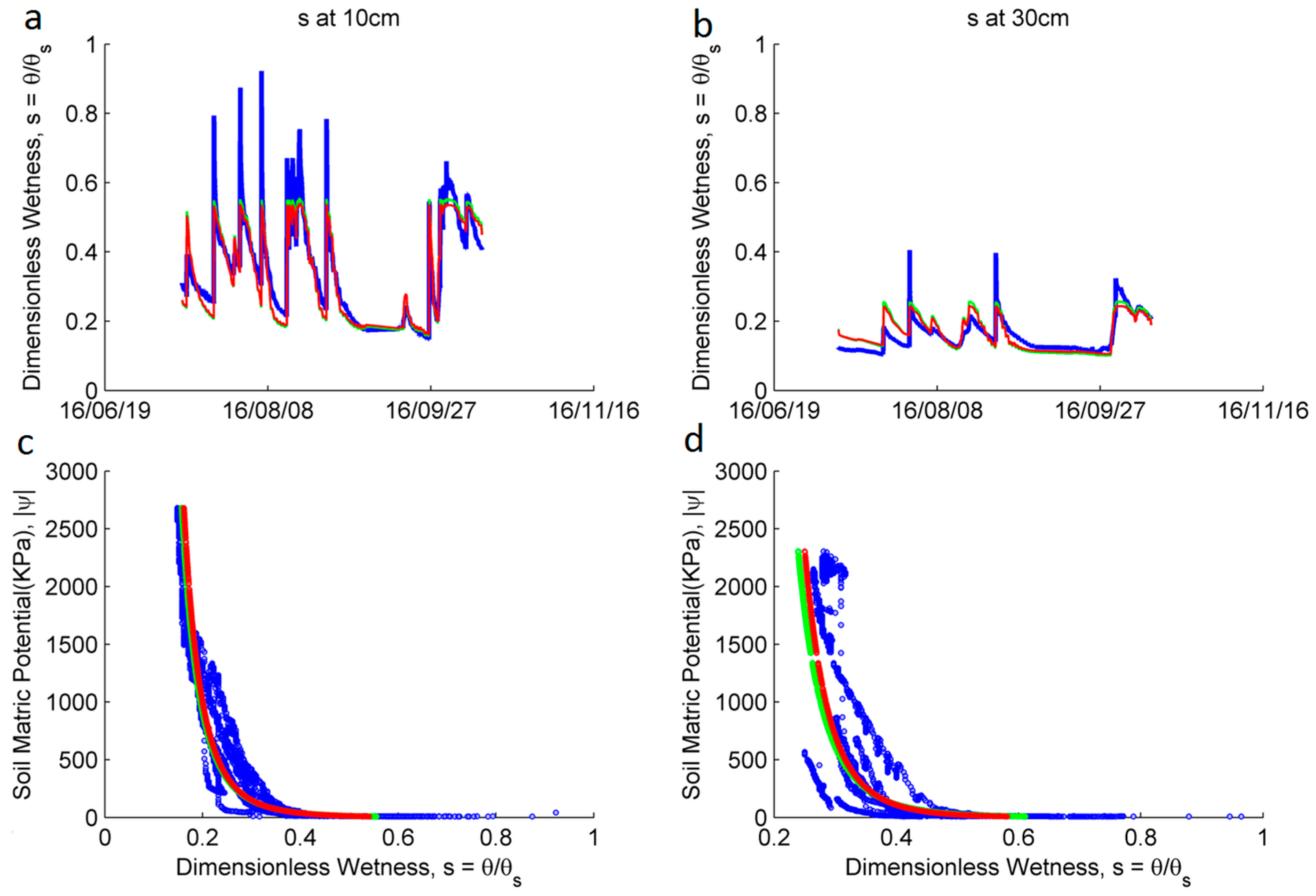
Figure 8 shows the empirical relationship between the SM,
, and the absolute value of the WP, in kPa, |
| at a depth of 10 cm and 30 cm for the location close to the middle of the hill (i.e., nodes 2282, 2292 and data logger DL2) in site 2. The fitted equations lead to similar results for both equations. At a depth of 10 cm the fitted parameter for the Clapp and Hornberger equation are:
= 0.658 kPa and b = 4.49; For the van Genuchten equation: n = 1.215 and
= 1.808. The porosity value
= 0.31 was calculated from a soil core taken in the same location. For the depth of 30 cm, the parameters for the Clapp and Hornberger equation are
= 0.521 kPa and b = 5.87; For the van Genuchten equation: n = 1.154 and
= 3.51. The porosity value
= 0.42 was calculated from a soil core taken in the same location.
Table 1 summarizes these results, including the location close to the lower part of the hill (i.e., Node 2262, 2272 and Data logger DL1). The fitted equations were evaluated using the Nash-Sutcliffe efficiency (NSE) [
85].
3.4. Exploration of Soil Moisture and Soil Water Potential: Spatiotemporal Trends
Determining and explaining the temporal and spatial hydrological patterns is one of the major challenges in the hydrological sciences, since the factors that control these patterns behave in a nonlinear way [
35]. In this study, a spatial analysis was performed in order to show the variability of SM and WP.
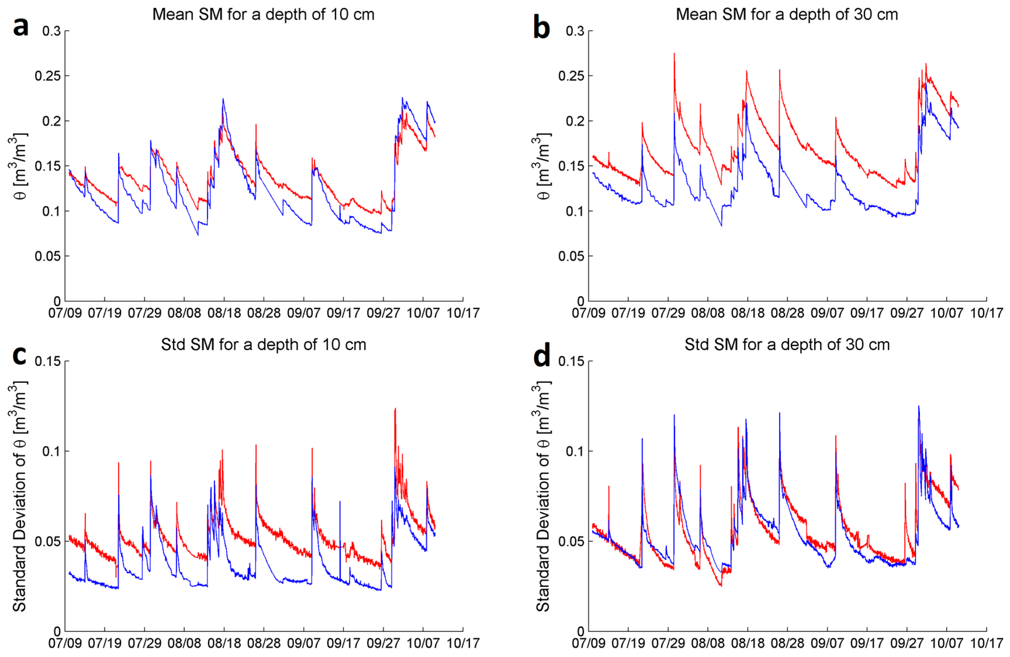
Figure 11 shows the time series of mean SM and its standard deviation at two depths (10 and 30 cm) for sites 2 and 6. The mean and standard deviation were calculated using hourly time series for each node in sites 2 and 6. Site 6 is characterized by a steep hill slope, while the slope is moderate for site 2.
Figure 11a,b show that the mean SM at both depths in site 2 is generally higher than that at site 6. The SM is especially higher at 30 cm (
Figure 11b).
Figure 11c,d show the standard deviation at sites 2 and 6, at 10 and 30 cm, respectively. It is shown that site 2 has a higher standard deviation than site 6, especially at 10 cm.
Figure 11 illustrates that, due to the presence of significant heterogeneity within a small spatial scale (e.g., the two sites are only a few meters away from each other), individual measurements (e.g., SM in this case) from the nearby locations can be quite different. To capture the variability of SM within a small spatial scale would require many sensors within an area of study. The traditional approach of connecting one or a limited number of sensors to a single data logger is not practical as it would require a large number of data loggers that would make the installation and maintenance cost prohibitive. In contrast, the WSN approach, together with the network protocol used here, makes such applications feasible as the cost is relatively low and data processing is centralized and simplified.
With these dense SM measurements, one can investigate scientific questions such as, how would the spatial variability of SM (both horizontally and vertically) affect evapotranspiration? To what extent, would the lack of knowledge of the spatial variability of SM lead to significant errors on hydrological modeling results? In addition, the WSN approach makes it possible to easily represent the time series of the mean SM patterns/trends for a small area that match a required spatial resolution needed for modeling studies.
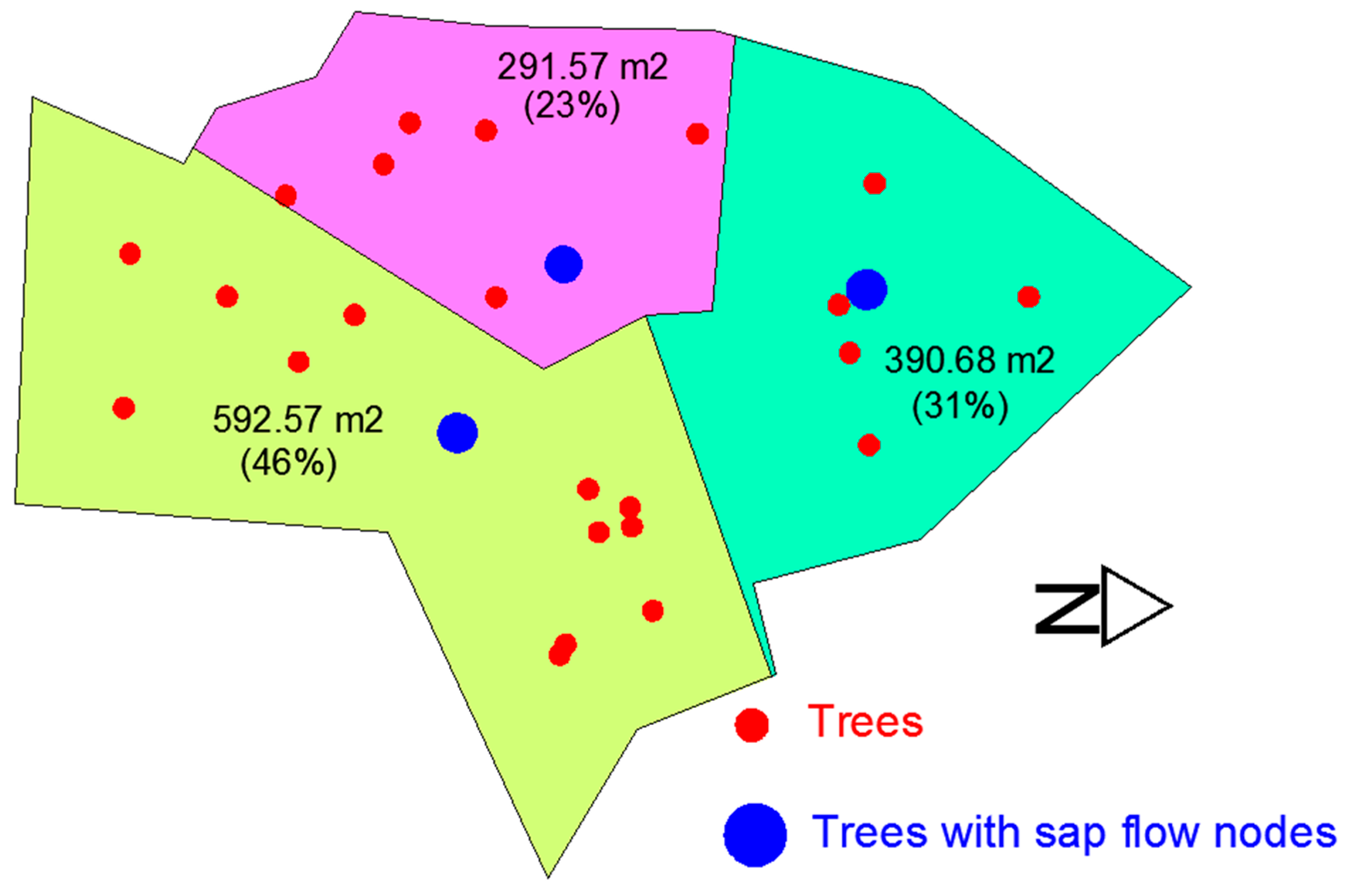
SM and WP surfaces (1-m cell size) were generated to illustrate the average spatial and temporal variability of these two parameters. The surfaces were built using the OK method. Along with the interpolated surface, elevation contours were generated from a 2-m resolution LIDAR raster, in order to complement the surface analysis by providing elevation input. The interpolation boundary was defined based on the area extent (approximately 15,000 m2) where the nodes are located. The highest and lowest elevations within the site are 365 and 346 m above mean sea level (m.a.m.s.l.), respectively.
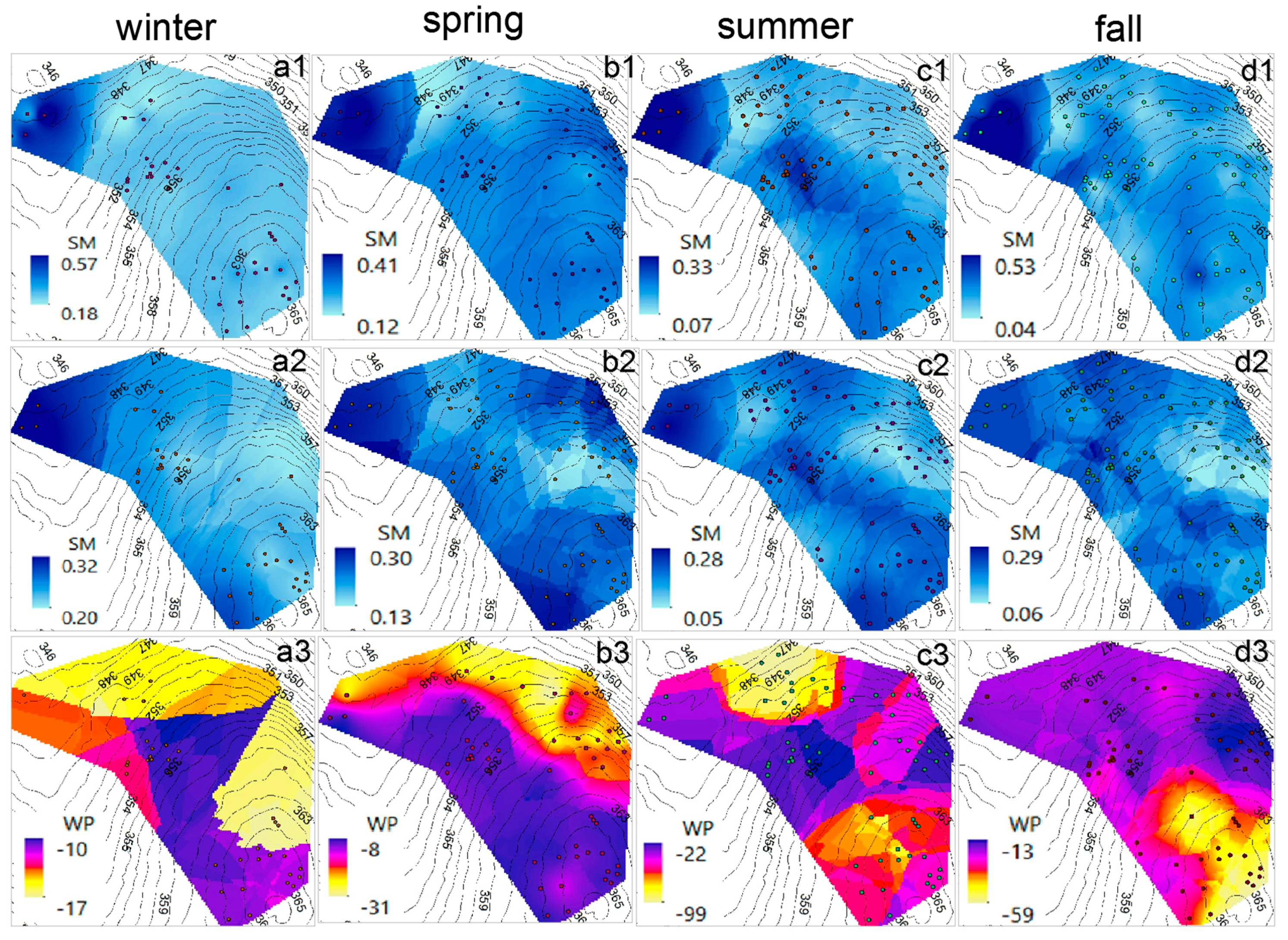
Figure 12 shows the average-seasonal SM (at 10 and 30 cm) and WP (at 30 cm) surfaces from 2010 to 2016. Overall, it is noticed that the higher SM area is located in the lower part (at 346 m.a.m.s.l.), within a flatter region near a pond. Also, it is observed that SM, regardless of the elevation, is more homogeneous during winter than in the other seasons, which might be caused by snow accumulation and melting over the winter. This is more evident in the average winter SM at 10 cm (
Figure 12a1), since the shallow soil is more influenced by the varying climatic conditions than the deeper soil [
90].
Another noticeable fact is that the average variation in SM is higher at 10 cm than at 30 cm, suggesting that the longer travel time to deeper soil reduces the spatial variability of SM. SM is lower during the summer than in the other seasons, which is consistent with the recorded daily rainfall data at the Pittsburgh Airport Meteorological Station [
91] for the 2010–2016 period, where there is a dry period between the end of the spring and summer months (i.e., May–September). Finally, based on the SM surfaces from summer and fall (
Figure 12c1,c2,d1,d2), there seems to exist a water pathway (darker color in the surface) from the highest elevation to the lower part of the area, located at the right side of the SM surface. This pathway might be explained by the natural surface and subsurface water movement towards the creek located to the south of the study area which, in turn, drains into the pond (immediately downstream of the region with higher SM). Topography showed stronger influence on SM during the winter. Regarding WP, the interpolated surfaces show a variable behavior from one season to another, but WP is mostly higher in the regions with higher elevations, even though there are some lower regions with higher WP.
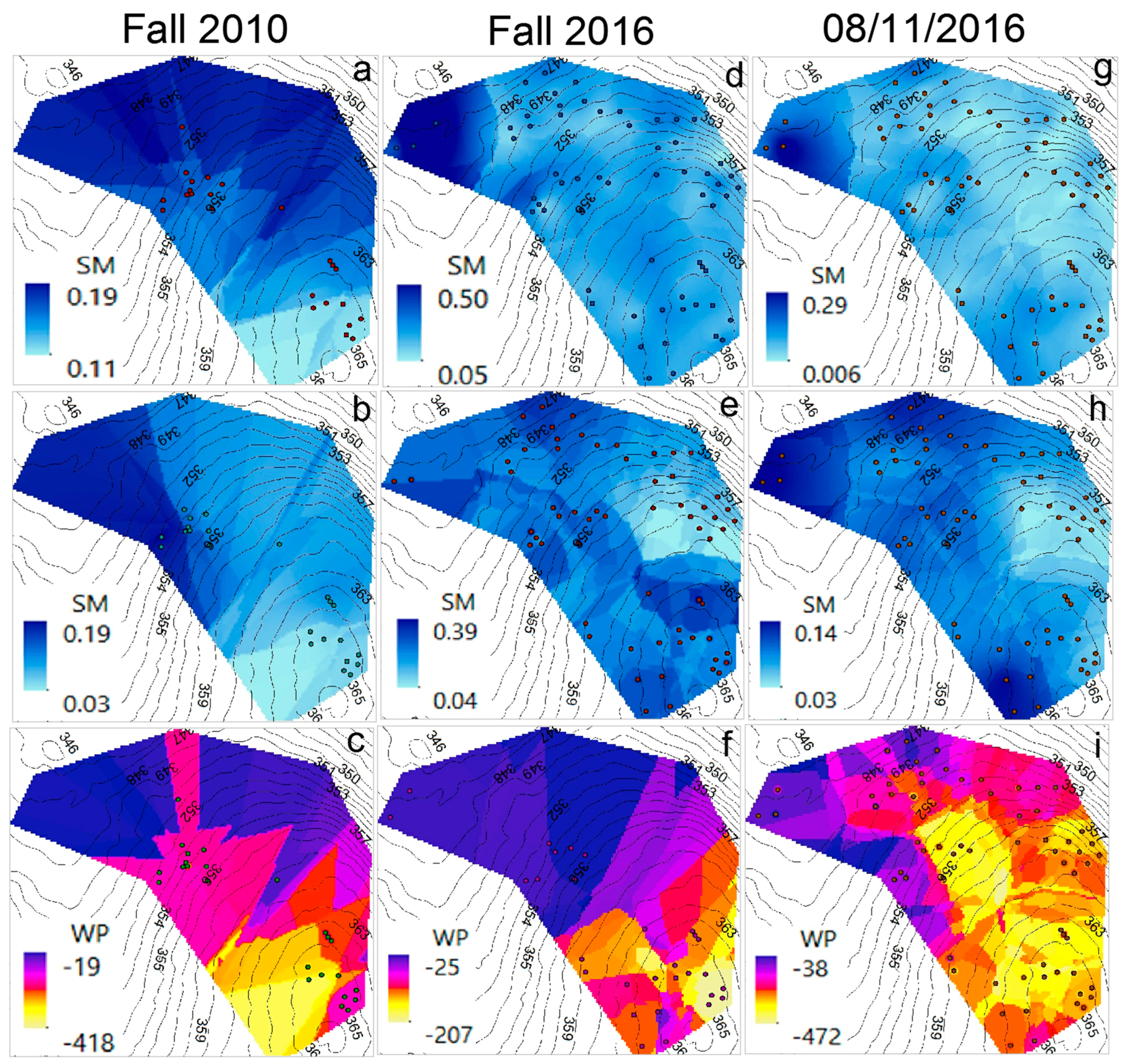
Figure 13 illustrates the improvement achieved by the network expansion. In highly complex and heterogeneous environments, the amount and quality of data is proportional to the amount of extractable knowledge [
92]. SM and WP interpolated surfaces were created for the average fall conditions in 2010 and 2016. Additional surfaces were generated for the average of 11 August 2016, which is the day with the highest recorded alive nodes (102 nodes, including the relays). In general, these surfaces show similar patterns for each corresponding variable (i.e., SM at 10 cm and 30 cm and WP at 30 cm). However, the 2016 network size, with less scattering in the node locations, provides better estimations than the 2010 network size. It is observed that the patterns for fall 2016 and 11 August 2016 are more similar to each other than the patterns for fall 2010 (see
Figure 13). This indicates that the higher node density in 2016 provides more detailed insights of the temporal and spatial variability of SM and WP. Overall, the analysis has shown the applicability of WSNs for short and long term hydrological patterns characterization at the catchment scale, for steep-forested environments.
In addition,
Table 4 shows the RMSE obtained from the OK interpolation for the scenarios presented in
Figure 12 and
Figure 13. The RMSE has the same units as the analyzed variable (i.e., SM or WP). The number of nodes from which the data was extracted, along with the maximum and minimum SM and WP values are also included. In terms of the SM, it is observed that RMSE is lower at 30 cm than at 10 cm, which is consistent with what has been shown before (i.e., that the SM is much more variable in the near-surface soil than in the deeper soil). In the case of the different average seasonal conditions, even with a different density of nodes within the site, the RMSE did not experience a significant change, thus showing the robustness of the OK interpolation method.
The lowest RMSE in SM, for both depths, obtained for 11 August 2016, suggests that a shorter period of time and a higher density of nodes reduce the uncertainty of the SM estimation. The estimated RMSE in the WP surfaces showed more variability than in the case of SM, mostly due to larger differences in the WP ranges for the analyzed conditions. However, if considering the error as a percentage of the range, the 11 August 2016 and fall 2016 average scenarios have the lowest percentages, 0.061% and 0.098%, respectively. In summary, geostatistical tools such as the OK interpolation constitute an important complement to WSNs for environmental monitoring purposes, especially when it is intent to estimate the spatiotemporal behavior of hydrological parameters.
3.5. WSN Challenges and Utility in Hydrology
There are several challenges faced in outdoor environmental monitoring WSN deployments, including power management, node maintenance, network scaling, heterogeneous deployment, and overall network cost [
93].
3.5.1. Power Management
It is of critical importance to maintain a constant power supply to the WSN nodes to ensure data collection and communication within the network. By far, the most common maintenance task is the replacement of batteries. Rechargeable nickel-metal hydride (NiMH) AA batteries were selected for powering the wireless motes as an environmentally friendly and cost-conscience means of maintaining the frequent battery changes of the network. Other alternatives such as the use of lithium-ion polymer battery (LiPo) were discarded due to budget constraints and the existing investment on a large number of AA (NiMH) batteries and chargers. Previous studies that analyzed the power efficiency of WSN motes using AA (NiMH) batteries showed that the expected autonomy of individual nodes is between 48 days [
94] and 58 days [
32]. More information about the energy profile for WSN nodes is available in [
95]. The use of solar panels has been considered, but, with the dense forestation surrounding the majority of the network, it did not appear to have a sufficient return on investment; although, it might be suitable for other locations with more exposure to direct sunlight or during the winter months following tree leaf senescence.
Despite the benefits of rechargeable batteries, some drawbacks exist. Following a recharge, the NiMH batteries may have a significantly higher voltage (e.g., 1.4 V). This leads to circumstances where the combined voltage of three NiMH batteries (i.e., 4.2 V) is significantly greater than the recommended safe operating voltage for the wireless motes (i.e., 3.3 V). Also, issues with irregular charging voltages were found in the NiMH batteries, which were sorted based on the recommended screening process described in [
32]. In order to maximize the life span of each relay node for each battery cycle, it is recommended using D batteries that have a capacity of about 10,000 mAh or more.
Over the span of the project, two sorting strategies were used for the batteries: full and partial sorting. In the full sorting strategy, before a maintenance event, all recharged batteries are sorted by their standing voltage from low to high. Replacement batteries are then chosen as consecutive groups of three from the sorted group. In the partial sorting strategy, batteries are grouped based their standing voltage into bins (e.g., 1.25–1.30 V). Replacement batteries for a single mote are then taken from the same bin. In this method, only voltage bins with an adequate number of batteries are used, which often leads to unused batteries in bins with only one or two batteries. In this regard, the full sorting strategy is slightly better; however, it is more time consuming. As indicated in Figure 16 of [
32], node battery life throughout the network improved following the adoption of a battery sorting strategy.
Another method for improving the battery life of wireless motes is to reduce its number of transmissions. This is due to the high-energy costs of transmitting wireless data [
94,
96]. During the first years of this project, each node had a sampling rate of 15 min. This was a trade-off between the desired sub-hourly temporal resolution of the environmental data, the expected battery life for each power cycle of the motes’ batteries, and the poor packet reception rate of the network, which was around 50% during the first years of deployment. With recent versions of the WSN protocol, the packet reception rate has significantly improved to over 90% [
32]. In addition, the new WSN protocol allows for the customization of network parameters for individual nodes according to their intended use. In order to reduce power consumption, the sampling rate of relay nodes (and some sensor nodes) was lengthened to 30 min. At the same time, to address measurement noise, the sampling rate for the sap flow nodes was shortened to 10 min. The increased sampling rate of the sap flow nodes was not a concern for battery life, as these nodes are powered by the 12 V lead-acid battery.
3.5.2. Node Maintenance
The maintenance of the data collection equipment depends on knowing the status of each individual node or data logger. However, the data loggers used in this study are not available on-line and therefore it is not possible to monitor the data collected with them in real time. In addition, in order to collect the data, the researcher needs to commute to the location where the data logger is located. There are some disadvantages with this approach. First, if a wire is loose, then data from one or several sensors attached to the data logger is lost. Second, if the batteries are depleted, then the data logger stops working. Third, there is no way to be aware of those issues until the data is downloaded and examined. Lastly, downloading the data from a data logger is time consuming and does not scale to the case of several locations because every location has to be downloaded independently. Also, the data for a single data logger generates a number of separate files (i.e., one at each location and time of downloading) that require further processing before analysis—as is the case for the Decagon Devices EM50 data logger used in this study. On the other hand, the data collected from our WSN is stored directly and automatically in a relational database that is available through a web-based integrated network and data management system for heterogeneous WSN site called INDAMS [
97] for online monitoring.
One way to reduce the need for node maintenance is by using enclosures of high quality, even though they tend to be more expensive, their associated costs pays off in the long run as they are more resistant to environmental damage, less prone to water intrusion, easier to open and close, and, therefore, easier to maintain. In addition, high quality enclosures keep the sensing and communication equipment, and the batteries safer.
3.5.3. Network Routing and Scaling
In multi-hop large-scale WSN networking, the routing protocol plays an essential role for reliably collecting sensor data in real time. While WSN deployments appear promising due to the limitations of traditional data logging methods [
98], the WSN scalability has proven to be a bottleneck in early studies. An increased network size introduces more data traffic, collisions and congestion in the network, resulting in network performance degradation. To mitigate this problem, starting from the summer of 2014, the ASWP network has adopted CTP + EER routing, which significantly reduces the workload of motes along efficient routes and thus extends the WSN lifetime.
During the network expansion, from 52 nodes in 2014, to 88 nodes in 2015, and finally to 104 nodes in 2016, the network performance has not been noticeably influenced while operating CTP + EER. The packet reception rate (PRR) of the network remains above 96%. The average packet path length is 3.95 hops during the 52-node network, 4.76 hops during the 88-node network, and 4.73 hops during the 104-node network. In the summer of 2015, both the width and length of the WSN deployment was expanded, which caused the increase of the average path length. In the summer of 2016, the major network change was its density, which caused a slight reduction in the average path length and PRR. This result demonstrates that with the proper routing protocol, the network is able to maintain high levels of performance over various deployment scales.
3.5.4. Heterogeneous Mote Reprogramming
The ASWP WSN deployment consists of three different mote platforms as well as multiple application versions (corresponding to various external sensors attached to individual motes). As an exploratory and evolving WSN deployment, the network application needs to be updated frequently to test new protocols and parameter configurations. Over-the-air reprogramming approaches become a natural choice since manually reprogramming the motes is cumbersome. The heterogeneous nature of the developed WSN with motes operating in LPL makes the existing reprogramming tools infeasible [
52,
53].
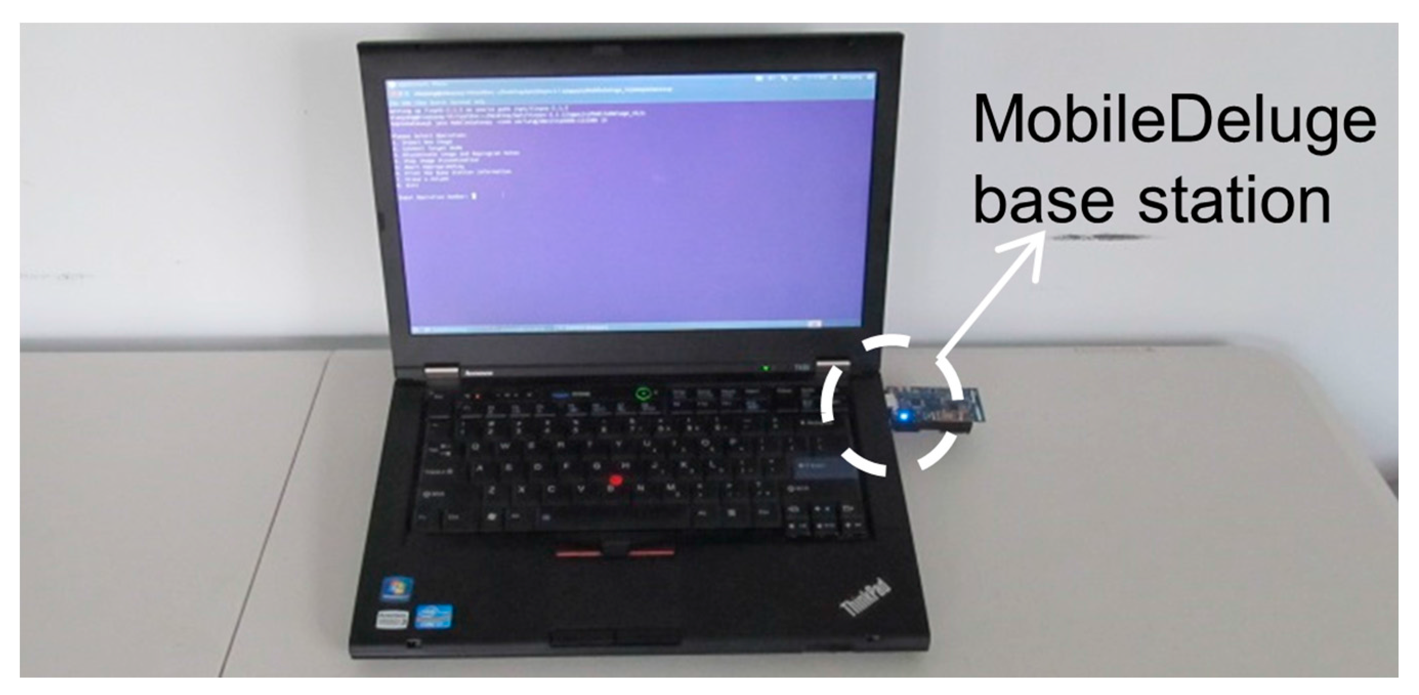
Our developed MobileDeluge [
52] is a novel hand-held mobile over-the-air mote reprogramming tool for outdoor WSN deployments (
Figure 14). MobileDeluge builds a new control layer on top of Deluge [
99]. It enables and disables Deluge services on demand, allowing for the selection of a subset of motes as targets when initiating a reprograming task. It then disables LPL in the targets for fast dissemination of the new application image, which usually consists of thousands of packets. The targets are also configured in a different radio channel to avoid interference with the rest of the network. MobileDeluge currently works with the motes within a one-hop range to avoid forwarding a bulk code image over intermediate nodes for mote energy conservation. Please see [
52] (and the references herein) for more details.
MobileDeluge has significantly reduced the time and labor required to update the application in the outdoor WSN testbed. The manual reprogramming procedure would consist of getting the enclosure from the tree, opening the box, attaching the mote to the laptop and uploading the new application. For example, it usually takes a few days to reprogram the whole ASWP testbed (i.e., 104 motes). With MobileDeluge, in contrast, the reprogramming can be finished within one afternoon.
3.5.5. Network Costs
The 52-node MICAz and IRIS network at the end of 2014 had a cost of $31,500 for the wireless motes, gateway, sensors, and other peripherals [
32]. The CM5000-SMA (TelosB) mote includes built-in humidity and temperature sensors and does not require the use of an acquisition board for relay nodes as opposed to the MICAz or IRIS motes that use the MDA300 acquisition board ($179). Therefore, the adoption of the TelosB motes has significantly reduced the cost of relay nodes, from $330 (in the MICAz network) to $164, despite the TelosB ($110) being slightly more expensive than the MICAz or IRIS motes (both models about $99 each). These savings are also found for the soil sensor nodes (from $664 to $480), mainly due to the deployment of our inexpensive ($13) designed sensor boards (with 5 V voltage booster) instead of the MDA300, despite the increased cost for the MPS-2 (compared to the MPS-1) sensor. A new sap flow box design, which replaced the MDA300 by our sensor board ($9) without the 5 V voltage booster and does not require the use of AA or D batteries, has further contributed to the cost savings (from $464 to $257). The cost of the expanded 104-node (27 MICAz, 32 IRIS and 45 TelosB motes) network is approximately $50,000.
Table 5 shows the distribution of sensors for each type of node.
For the sake of comparison, a Decagon Devices EM50 data logger costs about $476 and is roughly equivalent to our WSN soil sensor node ($177 without the sensors) in terms of its capability to host external sensors.


 ,
, 


