5.1. Communication Errors
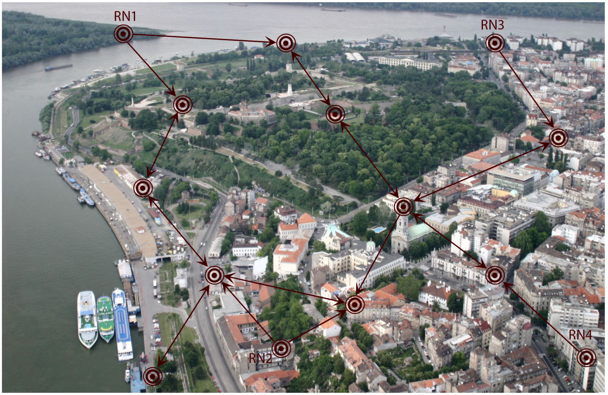
In this subsection, we assume that inter-node communication errors can be manifested in two ways: (1) communication dropouts (outages) and (2) additive communication noise. Communication dropouts typically occur in SNs using digital communication; additive noise can, in this case, model quantization effects. For example, in the case of smart city sensor networks, depicted in
Figure 1, the dropouts will happen relatively often because of the dynamic environment, where both physical obstacles and electronic interference can be persistent. In certain, less frequent practical situations, SNs can use analog communication (e.g., when certain types of energy harvesting are used [
56]), when additive communication noise is dominant, and dropouts appear less frequently.
The communication errors are formally introduced using the following assumptions:
(A5) The weights
in the algorithm (
5) are now randomly time-varying, according to stochastic processes given by
, where
are i.i.d. binary random sequences, such that
with probability
(
when
), and
with probability
.
(A6) Instead of receiving from the j-th node, the i-th node receives , where is an i.i.d. random sequence with and .
(A7) Processes , and are mutually independent.
Based on the above assumptions, the communication dropout at any iteration t, when node j is sending to node i, will happen with probability , independently of the additive communication noise process and the measured signal .
Denoting
and
, one obtains from (
10) that
where
, and
is obtained from
by applying (A5).
Convergence properties of the recursion (
20), under the additional assumptions (A5)–(A7), can be derived starting from the results of the previous subsection. Due to the mutual independence of the random variables in
, it can be concluded that
, where
is the same as
but with
replaced by
. Also, it follows that
, is a martingale difference sequence (since
). Furthermore, it can be concluded that
has the same spectrum as
in (
11): it has two zero eigenvalues and the rest eigenvalues are with negative real part.
Since the additive noise is now present in the recursions (
20), (A1) needs to be replaced with the following assumption, typical in the stochastic approximation literature (e.g., [
57]):
(A1’) , , , .
Intuitively, (A1’) introduces diminishing gains which converge to zero slowly enough, so that the additive noise can be averaged out while asymptotic convergence to a consensus point is achieved (despite the presence of noise).
Similarly as in the noiseless case, let as introduce the similarity transformation
where
is an
matrix, such that
. Then,
, where
and
are the left eigenvectors of
corresponding to the eigenvalue at the origin. By applying transformation
to (
21), and using stochastic Lyapunov stability arguments, along with the arguments typically used in analyzing stochastic approximation algorithms [
13,
17,
58,
59], the following theorem can be proved:
Theorem 3 ([
13,
17])
. Let Assumptions (A1’), (A2)–(A7) be satisfied. Then, generated by (21) converges to in the mean square sense and w.p.1, where and are scalar random variables satisfying and . The theorem essentially states that, again, all the corrected drifts converge to the same point, and all the corrected offsets converge to the same point; however, because of the additive communication noise, these points are random and depend on the noise realization. The mean values of these possible convergence points depend on the sensor parameters and , the design parameters , as well as on the dropout probabilities , .
5.2. Measurement Noise
In this subsection we, in addition to communication errors, assume that the signal
is measured with additive measurement noise. This situation is of essential importance for practical applications since practically all the existing sensors contain certain measurement errors which are typically modeled using stochastic processes [
3].
Formally, we model the additive noise stochastic process using the following assumption:
(A8) Instead of
given by (
1), the sensor measurements are now contaminated by noise, and given by
where
,
, are zero mean i.i.d. random sequences with
, independent of the measured signal
.
By replacing
instead of
in the base algorithm (
5), one obtains the following “noisy” version of (
8):
where
and
, assuming
,
. It is important to observe here that
,
; however
.
Assuming again that the step sizes
,
, satisfy (A1’), one can obtain the following equation analog to (
10):
where
and
with
for
and
for
,
.
In an analogous way as in the previous section, instead of (
11), the following equation is obtained for the mean of the corrected calibration parameters
where
is as in (
11) and
. Because of the additional term
, the sums of the rows of the matrix
are not equal to zero anymore, so that the convergence to consensus (as in Theorem 1) cannot be achieved in this case.
However, it can be seen from the structure of the recursion (
24) that, if we assume that the measurement noise variances
are a priori known, we can use them to modify the basic algorithm (
5) in the following way, ensuring again the asymptotic convergence to consensus:
where
and
,
.
The following theorem deals with the convergence of the above modification of the basic algorithm, when the measurement noise is present together with the communication errors. The convergence points will again depend on the measurement and communication noise realizations, in a similar way as in Theorem 3.
Theorem 4 ([
17])
. Assume that the assumptions (A1’), (A2)–(A8) hold. Then, , given by (25), converges to in the mean square sense and w.p.1, where and are scalar random variables satisfying and . Notice that the above theorem was based on assumption (A2): indeed, when both
and
are i.i.d. sequences, it is not surprising that the asymptotic consensus is achievable only provided
,
, are known. However, we can replace the unrealistic assumption (A2) with (A2’) (introduced in
Section 4 in the noiseless case) allowing correlated sequences
which is almost always the case in practice. In such a way, the correlatedness problem present in the algorithm (
24) can be overcame, without requiring any a priori information about the measurement noise process. The idea is to introduce instrumental variables in the basic algorithm in the way analogous to the one often used in the field system identification, e.g., [
60,
61]. Instrumental variables have the basic property of being correlated with the measured signal, and uncorrelated with noise. If
is the instrumental variable sequence of the
i-th agent, one has to ensure that
is correlated with
and uncorrelated with
,
. Under A2’) a logical choice is to take the delayed sample of the measured signal as an instrumental variable, i.e., to take
, where
. Consequently, we present the following general calibration algorithm based on instrumental variables able to cope with measurement noise:
where
and
,
,
. Following the derivations from
Section 3, one obtains from (
26) the following relations involving explicitly
and the noise terms:
where
and
In the same way as in (
23), we have
where
,
,
, where
for
and
for
,
.
To formulate a convergence theorem for (
28), the following modification of (A4) is needed:
(A4’) for some .
This assumption implies that the correlation
should be large enough. Similarly as in the case of (A4), it can be concluded that (A4’) implies that
is Hurwitz. Similarly as in the above cases, let as introduce the similarity transformation
where
is an
matrix, such that
. Then,
, where
and
are the left eigenvectors of
corresponding to the zero eigenvalue. The following theorem deals with the convergence of the instrumental variable algorithm (
26). The convergence point, again, depends on the noise realization.
Theorem 5 ([
16])
. Assume that the assumptions (A1’), (A2’), (A3), (A4’), (A5)–(A8) hold. Then , given by (28) with , converges to in the mean square sense and w.p.1, where and are scalar random variables satisfying and . 5.3. Asynchronous Broadcast Gossip Communication
So far we have shown how to deal with most of the practical challenges which emerge when dealing with real life SNs, such as communication dropouts, communication additive noise and measurement noise. However, in all of the above discussed algorithms we have implicitly assumed that all the nodes in the network share a common clock, based on which the recursions in (
5), (
25) or (
26) can be implemented synchronously. Indeed, when introducing the basic algorithm we have assumed that the signal
is being measured in discrete-time instances
t by all the nodes. These instances are also used as time indexes of synchronous recursions of the above algorithms. Yet, there are many practical cases of SNs for which it is impossible or impractical to function synchronously. A typical example is the case when the nodes follow certain slee** policies in order to minimize power consumption (e.g., [
3]). For example, the nodes in SN shown in
Figure 1, measuring air pollution or atmospheric conditions, may be programmed to make measurements less often during periods in which there is less traffic in the city. These types of situations are rigorously treated in the rest of this subsection.
Instead of the problem setup introduced in
Section 3, assume now that the sensors are measuring a continuous-time signal
at discrete points
,
,
,
, producing the sensor outputs
where the
and
are the same unknown parameters as in the previous subsections, and we also assume that the measurement noise
,
, is present in the sensor readings.
Furthermore, since the goal is to remove dependence on a common global clock, it is now assumed that every node
has its own local clock. For the sake of compact notation and simpler derivations, a single clock, called global virtual clock, is introduced, which ticks when any of the local clocks ticks. Hence,
in (
29) can be considered as the time in which the
k-th tick of the virtual clock happend. To have a well defined situation, it is formally assumed that the ticks of the local clocks are independent, and that the intervals between any two consecutive ticks are finite w.p.1. It is also assumed, for the sake of simpler derivations, that the unconditional probability that the
j-th clock ticked at an instance
is
, independently of
k. It is easy to verify that these conditions are satisfied for a typical model used in SNs, where it is assumed that the local clocks tick according to independent Poisson processes with rates
(as in, e.g., [
62,
63]). This case will be adopted throughout this subsection. It directly follows that, in this case, the virtual global clock ticks according to a Poisson process with the rate
.
According to the above assumptions, let us denote with the ticks of the local clock j, . The communication protocol can then be defined in the following way. At each local clock tick, a node j makes the local sensor measurement, calculates the corrected sensor output (based on the current estimates of calibration parameters and ), and broadcasts it to its out-neighbors . We assume also that communication dropouts can happen, i.e., each node receives the transmitted message with probability . For the sake of clarity of presentation, we do not treat additive communication noise in this subsection. It is also assumed that the communication delay is negligible, so that, practically at the same time instant all the nodes which have received the broadcast, perform the local sensor reading, calculate their corrected outputs , and update the local estimates of their calibration parameters and . This procedure is repeated for any local clock tick. The index of the node whose clock has ticked at instant is denoted by , and let be the subset of the out-neighbors which have received the broadcast message. Also, let , , , , , and for some l.
The measurement noise is treated as in the previous subsection, by using the delayed measurement
as the instrumental variable
where
is the global iteration number that corresponds to the closest past measurement of the node
i. By using the same local criteria as in (
3) and gradients as in (
4), the following new recursion for updating the calibration parameters at node
i is formulated:
where:
,
is the step size given by , where is the number of parameter updates of node i up to the iteration k, with ( denotes the indicator function),
, where
are the corrected outputs of node
and node
i.
The initial conditions are adopted to be . Note that, according to the problem setup, at a given iteration k only the nodes perform the above parameters update; for the rest of the nodes it holds that .
Computationally, the algorithm is as simple as the basic one, requiring only a few additions and multiplications in one iteration. Information needed at node i are: the local sensor measurement, the local instrumental variable, and the current output sent by an in-neighbor j. Knowledge of the global iteration index k (or ) is not needed.
From the above definition of the step size it can be concluded that it depends only on the number of local clock ticks, which makes the algorithm completely decentralized.
It should also be noticed that the instrumental variables in (
31) can be selected in several ways. For example, instead of choosing (
30), it can be practical to choose
, where
is the time instant of a supplementary measurement of node
i, just after the last step of the recursion (
31) has been locally performed. This scheme is not assumed in the sequel, because of much more complicated notation; all the results can be easily transferred to this case.
Similarly as in the synchronous case, we introduce:
and
Consequently, we have
where
and
where
, with the initial conditions
.
Recursions (
36) for
, can be written compactly as
where:
,
,
, with and for all , , otherwise,
,
, where and , for all , , otherwise.
The initial condition is .
Since we have formulated a slightly different problem setup than in
Section 3, we introduce a new set of assumptions, and denote them using letter B:
(B1) is a stationary random sequence, bounded w.p.1, and satisfying the ϕ-mixing condition.
(B2) Let , represent time instants in which node i performs measurements. Then, , where and , .
(B3) Graph has a spanning tree.
(B4) , , are zero-mean sequences of independent and bounded w.p.1 random variables. is independent of the process , with for all k.
Assumptions (B3) and (B4) are essentially the same as (A3) and (A8).
The
ϕ-mixing condition (B1) represents one of the strong mixing conditions, usually satisfied for sensory signals [
64,
65,
66].
Assumption (B2) represents an extension of the assumption (A4), adapted to the presence of the instrumental variable
in (
31). It guarantees the persistence of excitation in the sense that the variance of
must be greater than zero (for all
k, because of stationarity) so that constant signals are not allowed [
13,
55]. However, it also ensures sufficent correlation between the instrumental variable and the current measurement, so that e.g., white noise signals are also not allowed. It can be easily derived [
14] that (B2) is satisfied if the autocovariance function of
is positive in a sufficiently large interval around zero. Also, if the rates
are adjustable we can choose
large enough, such that (B2) is always satisfied. Therefore, (B2) is, in general, not restrictive for processes having dominant low frequency spectrum, which is typical in practical applications of SNs.
Based on the above modified problem definition, the following result was proved in ref. [
14], stating that both corrected gains and corrected offsets will converge to consensus points (which depend on the realizations of the stochastic processes) for all the nodes.
Theorem 6 ([
14])
. Let Assumptions (B1)–(B4) be satisfied. Then given by (37) converges to in the mean square sense and w.p.1, where and are random variables with bounded second moments. 
 ,
, 


