Since its development, extensive research on CP-ΦOTDR has been presented, including several studies discussing specific performance parameters (e.g., sensing range, maximum achievable sensitivity or dynamic range), thus characterizing and demonstrating the potential of the technique. However, the direct comparison of said works may not be straightforward, since different measurement settings and/or optical components were used. For example, the reader may wonder whether the maximum sensitivity may be achieved for the maximum sensing range, or whether the CRLB is achievable for lower digital samplings or with different optical filters.
Experimental Setup
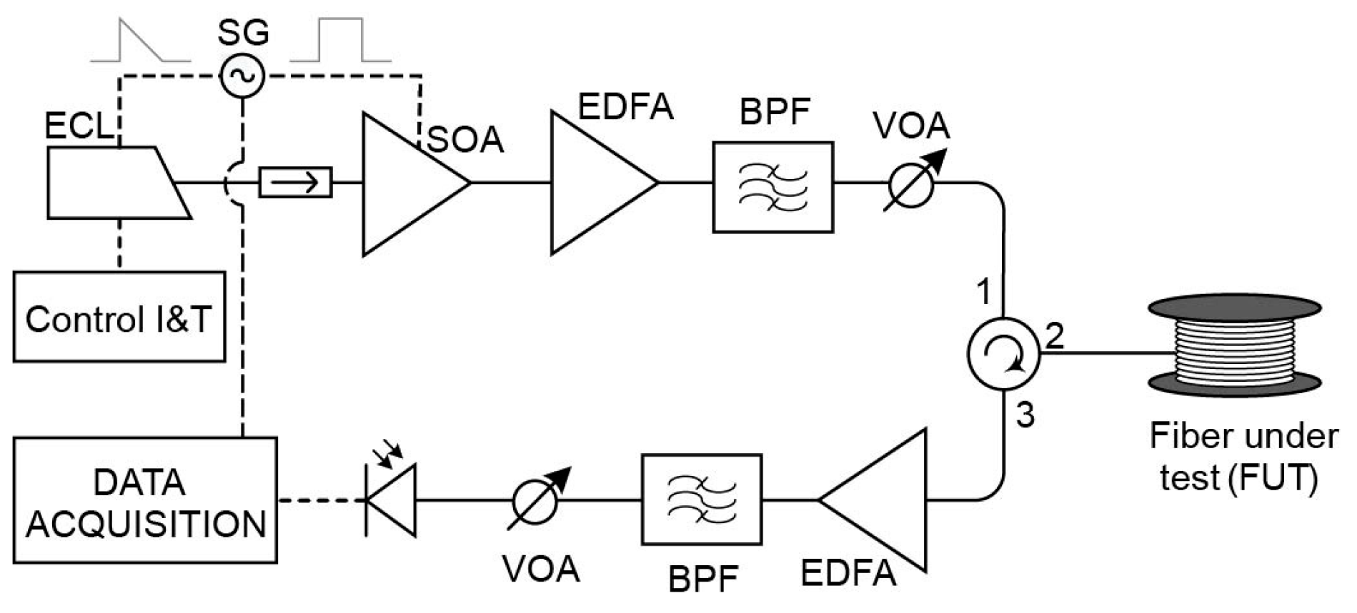
The experimental setup (
Figure 17) is based on that of the initial CP-ΦOTDR demonstration [
10]. An external cavity laser (ECL), with 1 MHz linewidth, operating in continuous emission is used as light source. The laser central wavelength is 1550 nm (
= 193.40 GHz), controlled by an external current and temperature controller. A secondary current control is used to introduce repetitive current ramps, thus introducing a periodic linear chirp in the outputted laser light. The laser output light is then pulsed in the time-domain using an SOA with nominal 50 dB extinction ratio and rise/fall times in the order 2.5 ns, fed with rectangular-like electrical pulses synchronized (same signal generator) with the laser chirp ramps. The pulse repetition rate (
) is 1 kHz, allowing measurements of up to ~100 km of fibre (Equation (7)). The output optical pulses present a 100 ns FWHM (
—setting a spatial resolution of 10 m) and 400 MHz spectral content (
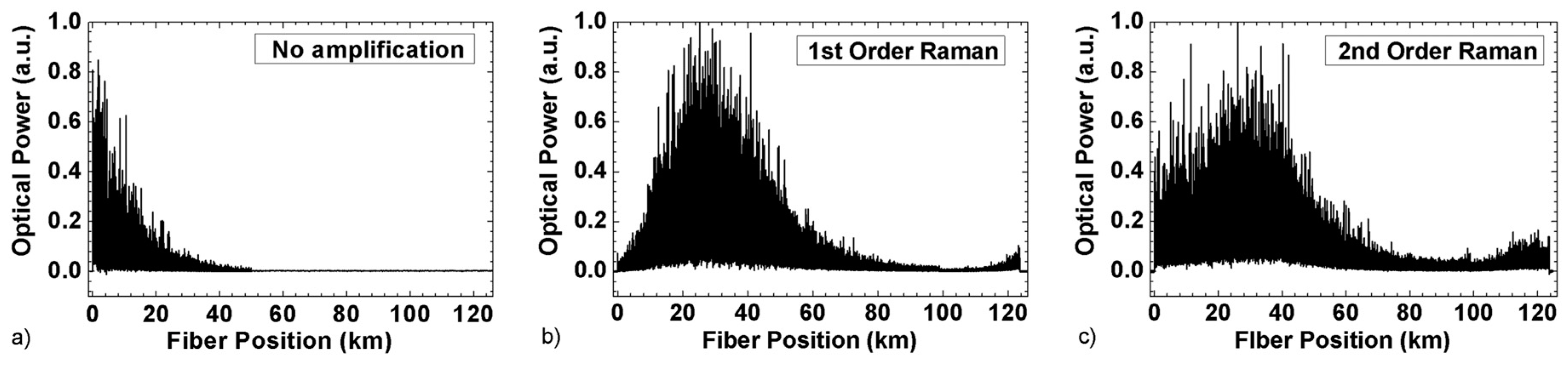
). An amplification stage composed of an EDFA, a 100 GHz standard dense wavelength division multiplexer (DWDM) (used as BPF), and a VOA is used to control the pulse peak powers before launching then into the FUT via an optical circulator. For the experiment, three FUTs are used with 50 km (single 50 km fibre roll), 75 km (50 km + 25 km fibre rolls), and 100 km (50 km + 50 km fibre rolls) of SMF. A calibrated piezoelectric (with a length of 60 m) is used to apply sinusoidal strain signals of known amplitude. The setup allowed the possibility of using distributed Raman amplification (with no amplification, co-propagating amplification or bi-directional amplification) with the use of the Raman pump lasers (emitting at 1455 nm, allowing pump powers of up to 400 mW each), coupled to the FUT via 1450/1550 WDMs [
27]. Another amplification stage (composed of an EDFA, a 100 GHz standard DWDM, and a VOA) was used to amplify the FUT Rayleigh backscattered light, before reaching the photodetector (520 MHz bandwidth p-i-n). The optical trace was recorded with a 1 GS/s digitizer and processed by a commercial GPU. All data was processed in real-time, aiming at demonstrating the practical feasibility of the sensor, and streamed to an external disk via a common USB 3.0 port.
With respect to previous experiments the cost/complexity of the system was greatly reduced while maintaining the high performance of the sensor. The sensor did not require [
12] the use of high coherence lasers (replaced by low coherence laser using laser noise compensation [
11]) and/or external modulator controlled by an arbitrary waveform generator (AWG): the laser was directly modulated in current. The BPFs are low-cost commercially available and the use of high sampling rate digitizer was avoided (1 GS/s with digital interpolation [
12], replacing the 40 GS/s used for the initial concept demonstration [
10]).
With the sensor presented in
Figure 17, the optical traces and strain variation signals were recorded for all positions of the fibre during a statistically significant time (2–5 min), allowing for distributed characterization of trace SNR and strain noise/sensitivity characterization along the entire fibre link.
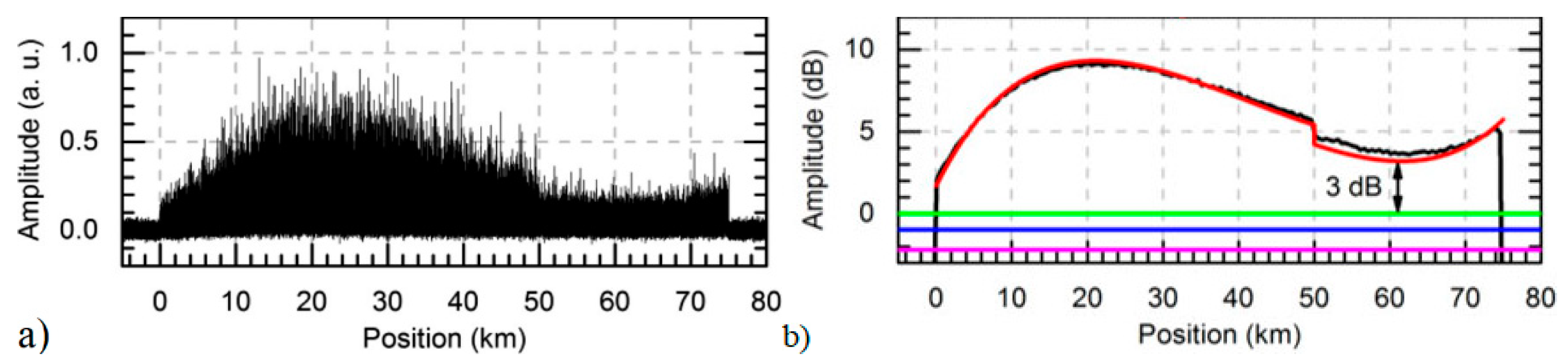
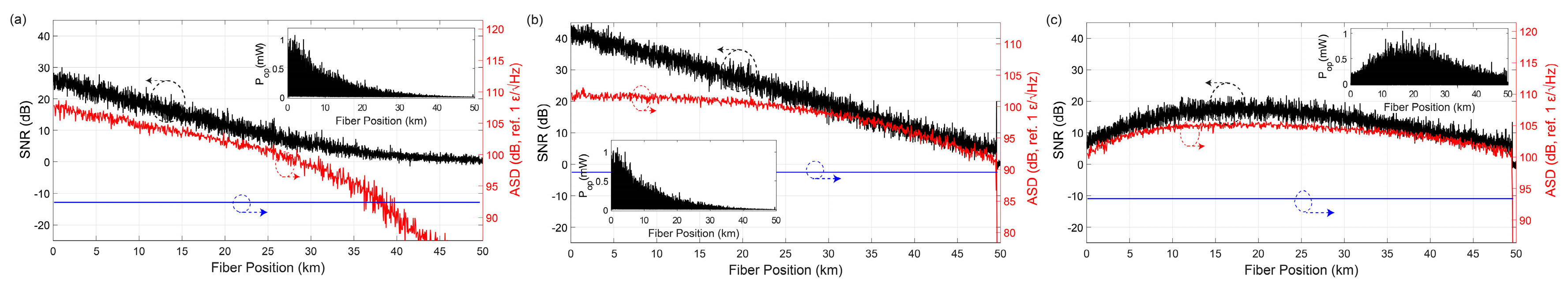
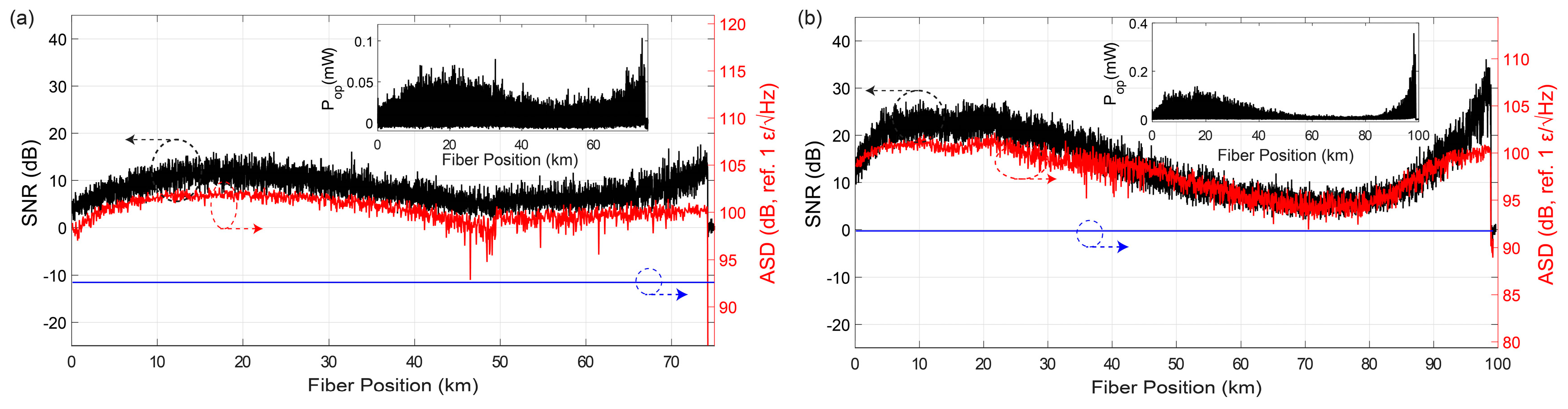
Figure 18 shows the results for a 50 km fibre measurement with three different measurement parameters (see figure caption for details). The trace electrical SNR (
—black line) is computed by using the variance of the photodetected signal before the beginning of the trace as the noise level (N) and the photodetected trace power along 10 m windows (i.e., equal to the used correlation window
, thus matching the sensor spatial resolution) as signal (S) [
45].
The figure also shows the strain ASD noise floor (
—sensor’s sensitivity noise floor) in each case (red line, inverted, for visual comparison with the
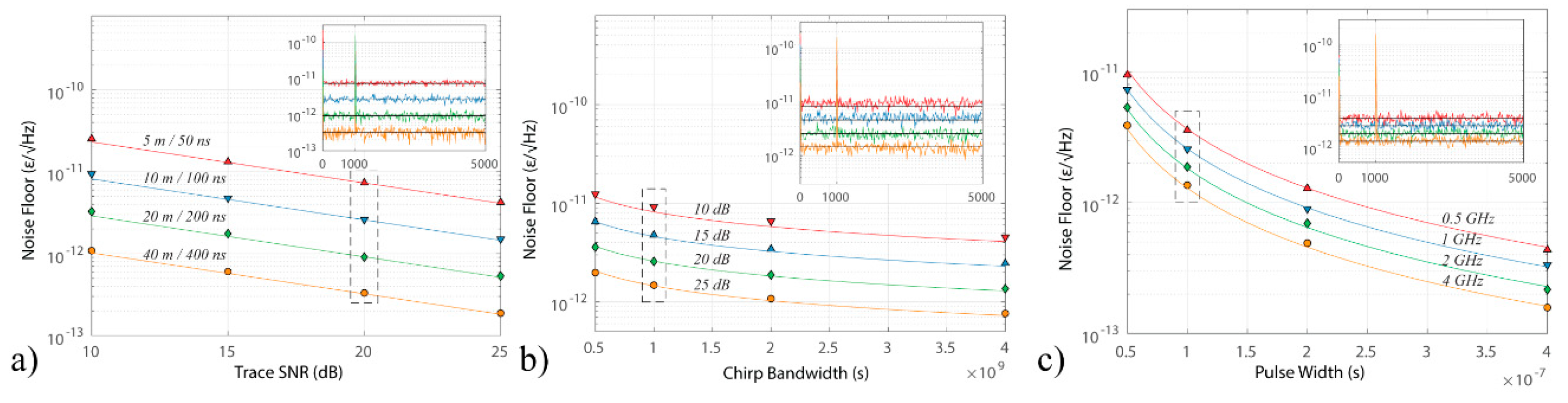
). With the used configuration, the theoretical CRLB limit for strain
(see Equations (12) and (13), see [
12]) is:
The offset and scale between the axis of the and strain are adjusted so that the theoretical CRLB limit of strain would be the overlap of the red and black curves (according to Equation (17)). For an easier visualization, the results are presented in logarithmic scale and referenced to 1 pε/√Hz, using: (e.g., ).
A few comments can be made to the presented results. The similarity of the red and black curves (in terms of absolute value, as well as variation along the fibre), demonstrates that the presented CP-ΦOTDR is well conditioned, operating with performance levels close to the theoretical CRLB limit level. Regarding
Figure 18a, a sensitivity of 15 pε/√Hz is achieved at the fibre beginning and the sensing range is limited to ≈35 km (note that the noise increases rapidly after this point) due to the occurrence of large errors when the trace SNR falls below a certain level. In any case, the robustness of the TDE via use of correlations in CP-ΦOTDR is well demonstrated, allowing operating with 100 pε/√Hz, even when the trace
is as low as 3 dB (for this configuration; note that operation below 0 dB SNR is possible for larger chirps
and/or correlation windows
). Regarding
Figure 18b, it is observed that the sensing range can be extended with the use of trace (temporal) averaging, as the entire 50 km of FUT is measured. The averaging is performed by acquiring and averaging the photodetected signal of N (=40) consecutive traces before performing the TDE (i.e., strain calculation). Note that in this case the frequency response of the system is changed, as averaging will act as a low pass filter in the acoustic response, i.e., there is a trade-off between acoustic bandwidth and sensing range. The improvement of the strain
for increasing trace SNRs saturates when
, (red line deflects from theoretical CRLB close to the fibre beginning), indicating the presence of additional residual noises in the system. With the use of distributed amplification (
Figure 18c), the performance along the 50 km is homogenized, with the strain
being keep above 100
in all fibre. With the use of averaging (without Raman)—
Figure 18b—or Raman (without averaging)—
Figure 18c—the sensing range is extended beyond 50 km.
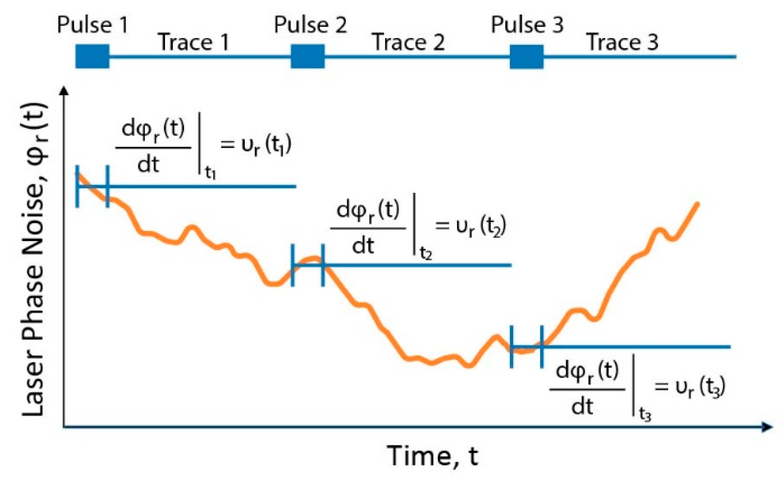
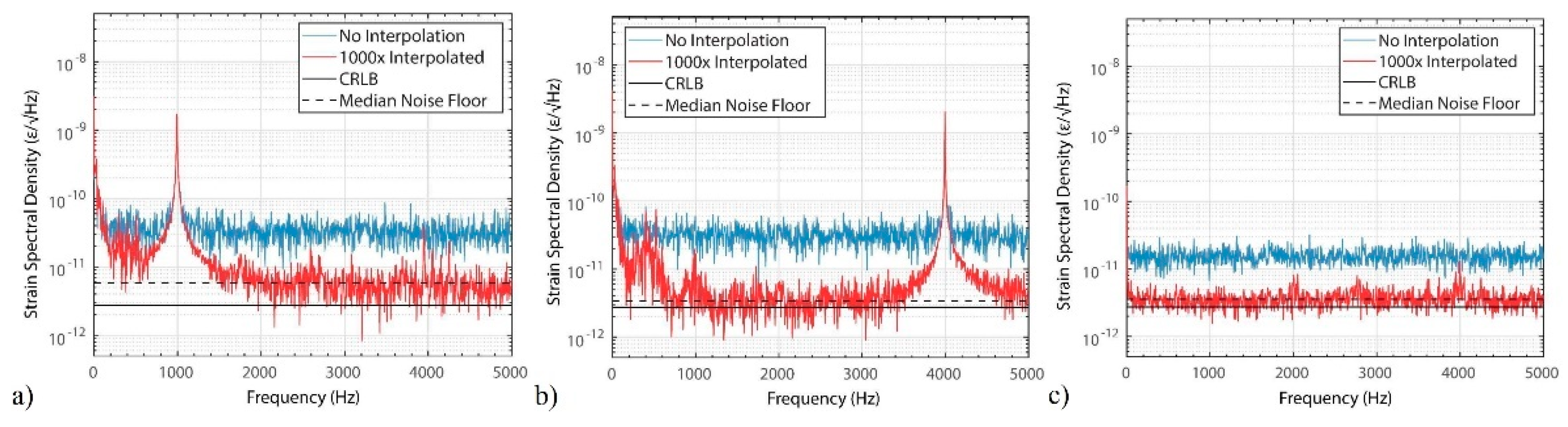
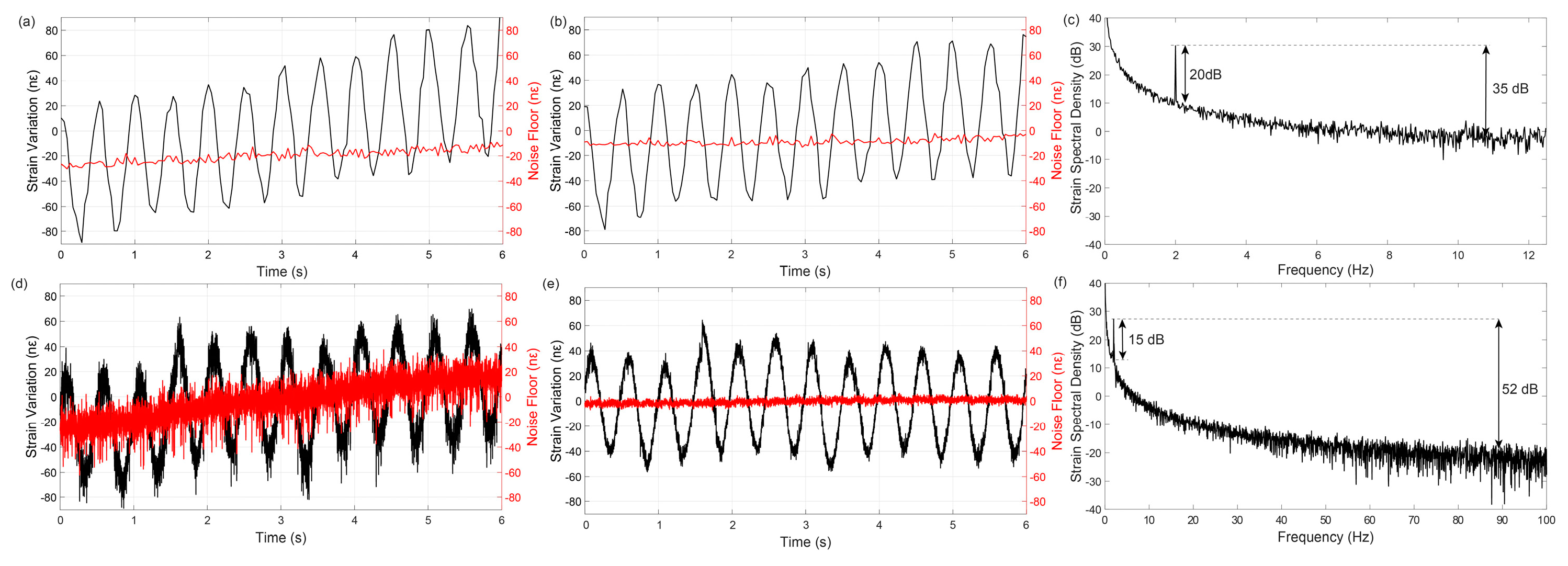
The laser noise level, (i.e., the strain noise level of the measured signal before compensating the laser noise) is presented in blue, demonstrating the effectiveness of the technique [
11]: an improvement of up to 15 dB in strain
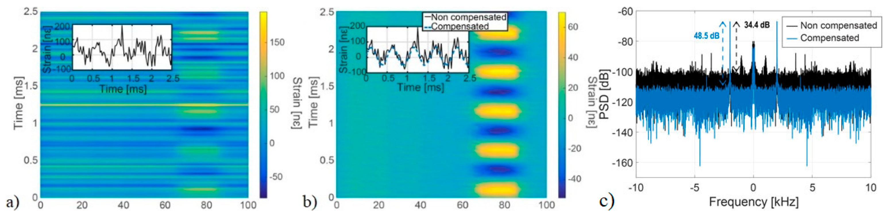
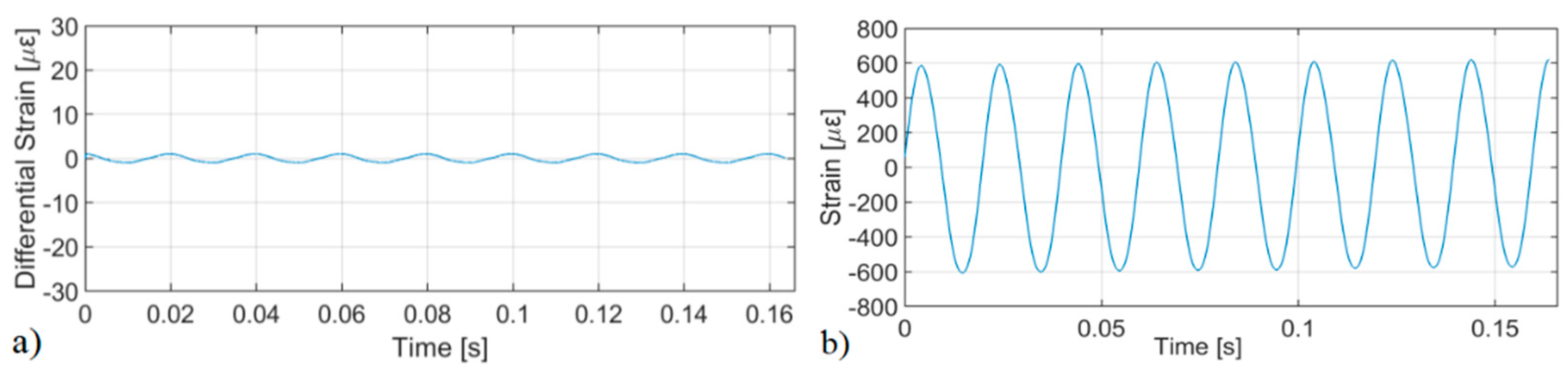
(i.e., 30 dB in strain PSD) is achieved by compensating the laser noise. This improvement (as well as a demonstration of the performance of the sensor after 50 km of fibre) is also shown in
Figure 19: a 2 Hz sinusoidal strain signal with 80 nε peak-to-peak applied by the piezoelectric is displayed before and after the laser noise compensation. Small but noticeable temperature drifts are also observed. See Figure caption for details. By computing the PSD of the strain signal, an SNR of 20 dB for configuration of
Figure 18b (presented in
Figure 19c) and an SNR of 15 dB for configuration of
Figure 18c (presented in
Figure 19f) is measured for this perturbation. However, it should be noted that the acoustic SNR at this frequency (2 Hz) is impaired by the existence of 1/f noise in the measurement (see
Figure 20 for further details on this noise). Perturbations of similar amplitude at higher frequencies would yield an SNR of up to 35 dB and 52 dB, respectively, as depicted.
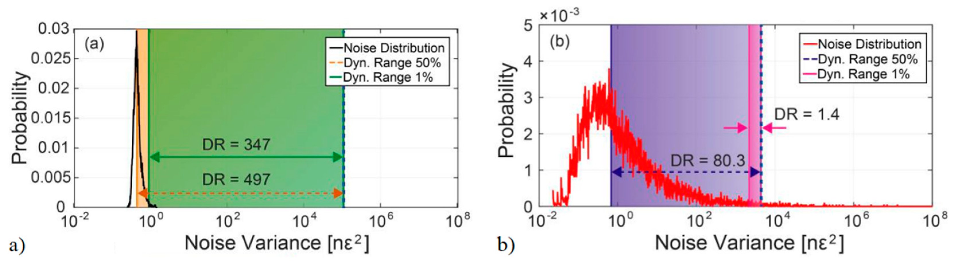
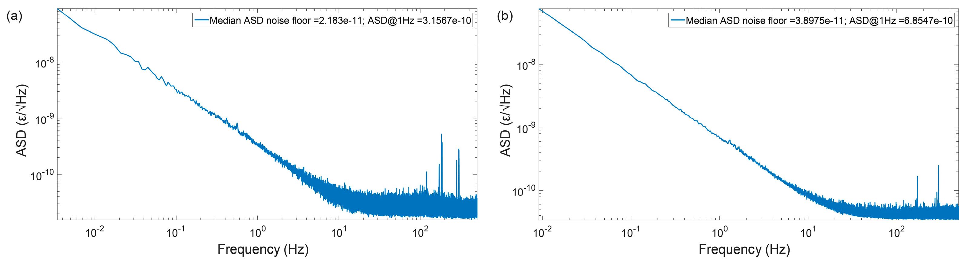
Figure 20 shows the strain ASD distribution, for the first 10 km of fibre (of configuration of
Figure 18a) and for the entire 50 km of fibre (of configuration of
Figure 18c). Note that the results show the average statistics for all the fibre points (in the considered section), during 5 min. As expected, the best performance can be achieved at the beginning of the fibre, where the trace SNR is higher (
Figure 20a), but with the use of distributed amplification the performance is homogenized along the fibre, achieving a high performance along the entire 50 km (
Figure 20b). A strain ASD noise floor of 22 pε/√Hz (
Figure 20a) VS 39 pε/√Hz (
Figure 20b) is demonstrated at high frequencies. At lower frequencies (of relevance for e.g., seismic applications), a 315 pε/√Hz (
Figure 20a) VS 685 pε/√Hz (
Figure 20b) is demonstrated at 1 Hz.
Note that the main difference when comparing to the results of
Figure 20a to [
12] (over 10 km) is the use of a lower trigger rate (
= 1 kHz here VS 10 kHz in [
12]), but the performances are comparable.
While an extensive discussion on the existing 1/f noise at low frequencies is out of the scope of this paper, it should be noted that the measurement was not performed in a thermally stabilized environment (i.e., it is unclear if this measurement is partially impaired by environmental noises at said frequencies, and not only the noise of the measurement technique).
The possibility for long range measurements is characterized in
Figure 21, where the trace
VS strain
is computed along the FUT for 75 km and 100 km, using bi-directional Raman amplification (details in figure caption).
The sensor strain is maintained above 150 pε/√Hz and 400 pε/√Hz, respectively (corresponding to a strain standard deviations of ≈3.3 nε and ≈2 nε, see Equations (13) and (17)) in the worst SNR point of the fibre in both cases, which demonstrated the high sensitivity of the sensor even for long ranges.


