In this section, we present both a quantitative and a qualitative analysis of the results, obtained with identical CNN predictors trained on various datasets. In addition, we compare our findings with previous research conducted on depth images [
13]. We split the following sections into three parts. First, we analyze the results obtained on grayscale and color images, also denoted as 2D images. We then discuss the
Fixed z-axis parameter limitation and ways to solve it. Next, we compare our method with the state-of-the-art method by Paschalidou et al. [
10]. Finally, we observe how well our predictors, trained on artificial data, perform on real-life images.
4.5.1. Reconstruction from 2D Images
Results with Intensity Images. The first set of experiments aims to evaluate the performance of our ResNet-18 model on regular intensity images and compare it to the performance on depth images, to determine whether superquadric recovery is also possible from images that lack spatial information. To ensure a fair comparison with previous work, we made sure that our generated depth images closely resembled those of Oblak et al. [
13] and retained the same renderer setup for intensity images. In addition, we generated both datasets using the same superquadric parameters.
By simply comparing the IoU values from the first two rows in
Table 1, it is clear that the model trained on intensity images with no restrictions (
Intensity (
Free z)) performed considerably worse than the one based on depth images (
Depth), with the latter scoring 0.387 higher on average. This large discrepancy can be attributed to the enormous errors made when predicting the
z position parameter. Predicting these values is virtually impossible, at least in the given setting, considering the camera perspective and the superquadric coordinate system. For example, identical images can be obtained with a smaller superquadric placed closer to the camera and a larger superquadric placed further away. This issue, in turn, noticeably affects predictions of other parameters, because the model does not converge properly. Furthermore, this showcases the difference in difficulty between the given task and the one tackled in previous work by Oblak et al. [
13].
To combat this issue, without altering the image generation process, we trained our predictor on a dataset of intensity images with a
Fixed z position parameter (
Intensity (
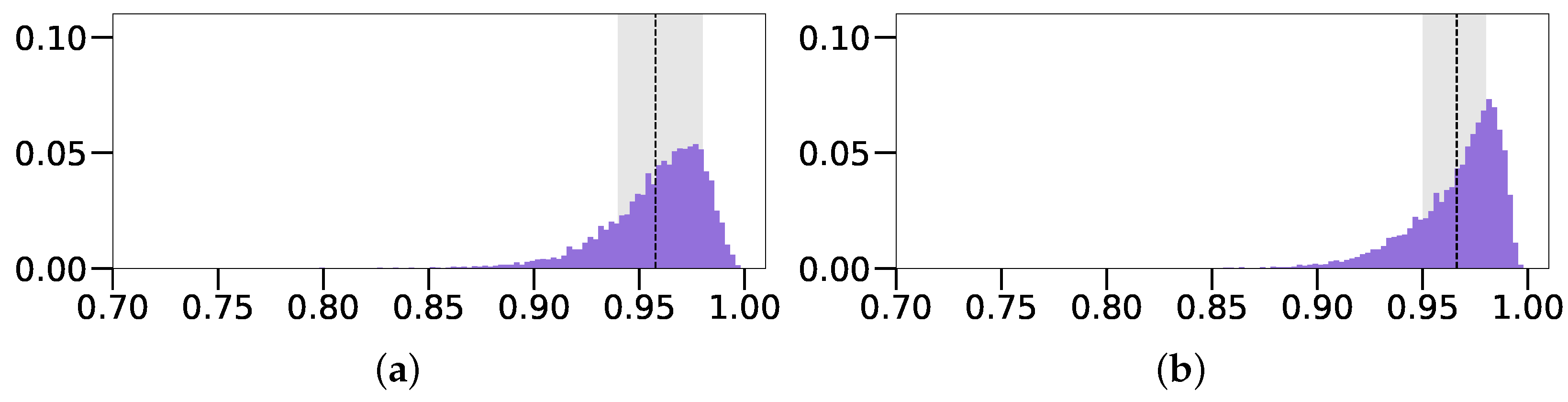
Fixed z)), meaning that it was set to a fixed value across the dataset. With this configuration, our model achieved considerably better performances across the board, in terms of all MAE parameter values and IoU accuracy. It even slightly surpassed the model trained on depth images, which can more clearly be seen in
Figure 8, where we see that the distribution of the intensity-based model has a much higher peak and smaller standard deviation range. Its mean IoU value of 0.966 was also slightly higher compared to the 0.958 of the depth-based model of Oblak et al. [
13]. In addition, we observe rather low standard deviation values overall, which suggests that the predicted parameters are fairly close to the ground truth for the majority of images. However, this performance comes at the expense of not being able to predict the
z position parameter, which negatively affects the capabilities of the trained CNN predictor.
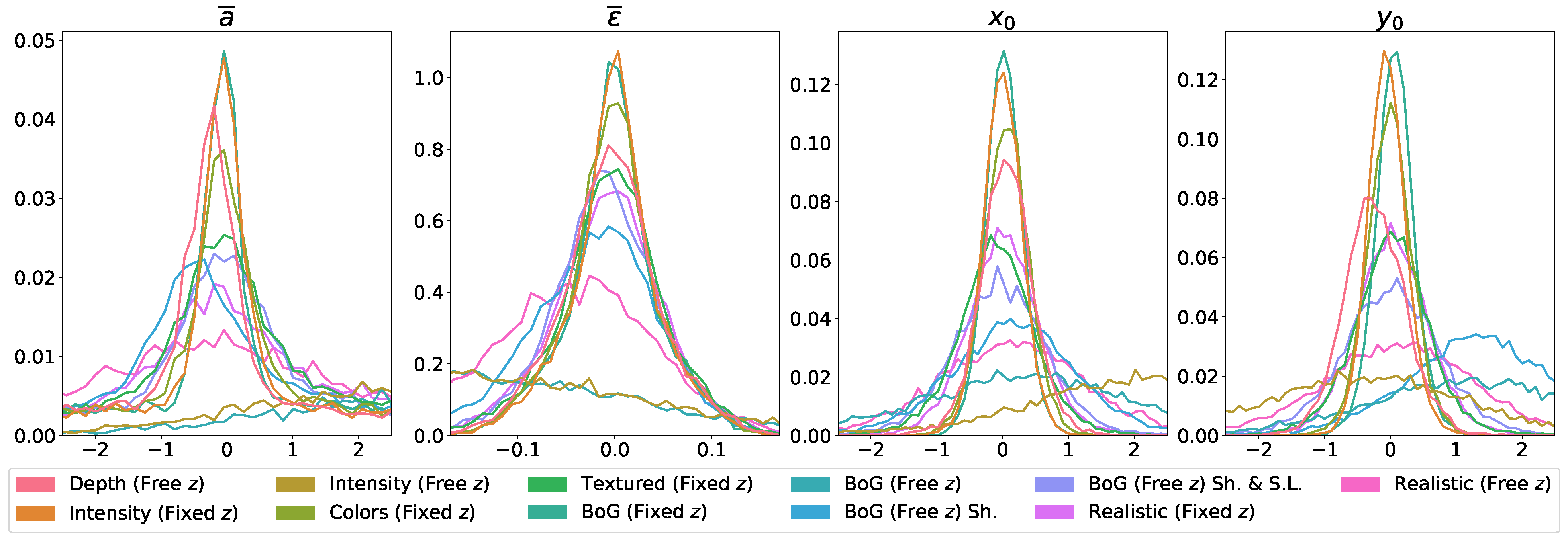
By analyzing the error distributions in
Figure 7, we observe that both
Depth and
Intensity (
Fixed z) models have rather Gaussian-like error distributions for all parameter groups, centered around an error of 0, exhibiting stable behavior. In comparison, the model based on intensity images with an unlocked
z parameter (
Intensity (
Free z)) exhibits rather unstable behavior with non-Gaussian error distributions that are heavily skewed in either the negative or positive directions.
From this experiment, we conclude that superquadric recovery from intensity images can be just as successful as recovery from depth images [
13]. However, this is only true if some form of additional spatial information is provided, such as the
Fixed z position of superquadrics in space, which determines how far away from the camera the object is. Without this constraint, the position of the superquadric becomes ambiguous and, thus, drastically affects performance.
Results with Color Images. Having showcased that superquadric recovery is possible from intensity images, we now focus on the reconstruction from color images. The following experiments aimed to explore how the complexity of color images affects the performance of our CNN predictor.
We begin with a model trained on images with uniformly colored superquadrics and backgrounds, whose superquadrics follow the
Fixed z parameter constraint as discussed before, denoted as
Colors (
Fixed z). The model achieves an IoU score of
, which is only slightly worse than the ones of the
Intensity (
Fixed z) model (
). However, it still performs slightly better than the depth image-based model (
) [
13]. The
Colors (
Fixed z) model also performs slightly worse than the intensity image-based model in terms of MAE scores of all parameters. However, the differences are rather negligible, especially for the shape and position parameters. Thus we can conclude that additional colors and colored backgrounds do not noticeably impact the performance of the predictor, despite the background and superquadric sometimes matching in color.
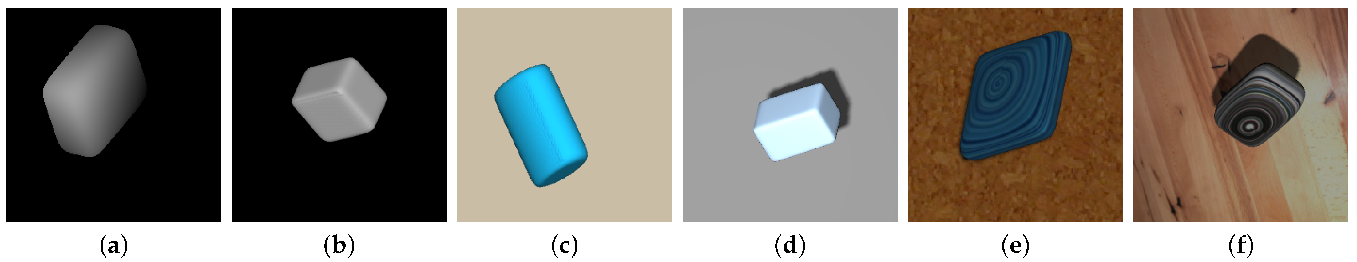
Next, we increase the complexity of the images by using randomly textured superquadrics and backgrounds, an example of which can be seen in
Figure 5. Analyzing the results, we observe a decrease in performance across almost all metrics. The accuracy of the
Textured (
Fixed z) model (
) is considerably worse than that of the previous model (
Colors (
Fixed z)), both in terms of mean and standard deviation. The same is true for most shape and position parameters. Interestingly, we observed an improvement in the MAE scores for the size parameters, possibly due to the trade-off between parameters. Overall, the obtained results show that our simple CNN predictor remains highly successful, even on significantly more complex images of superquadrics. Despite the performance being slightly lower than that achieved on intensity and color images, it is still acceptable and comparable to the initial performance on depth images.
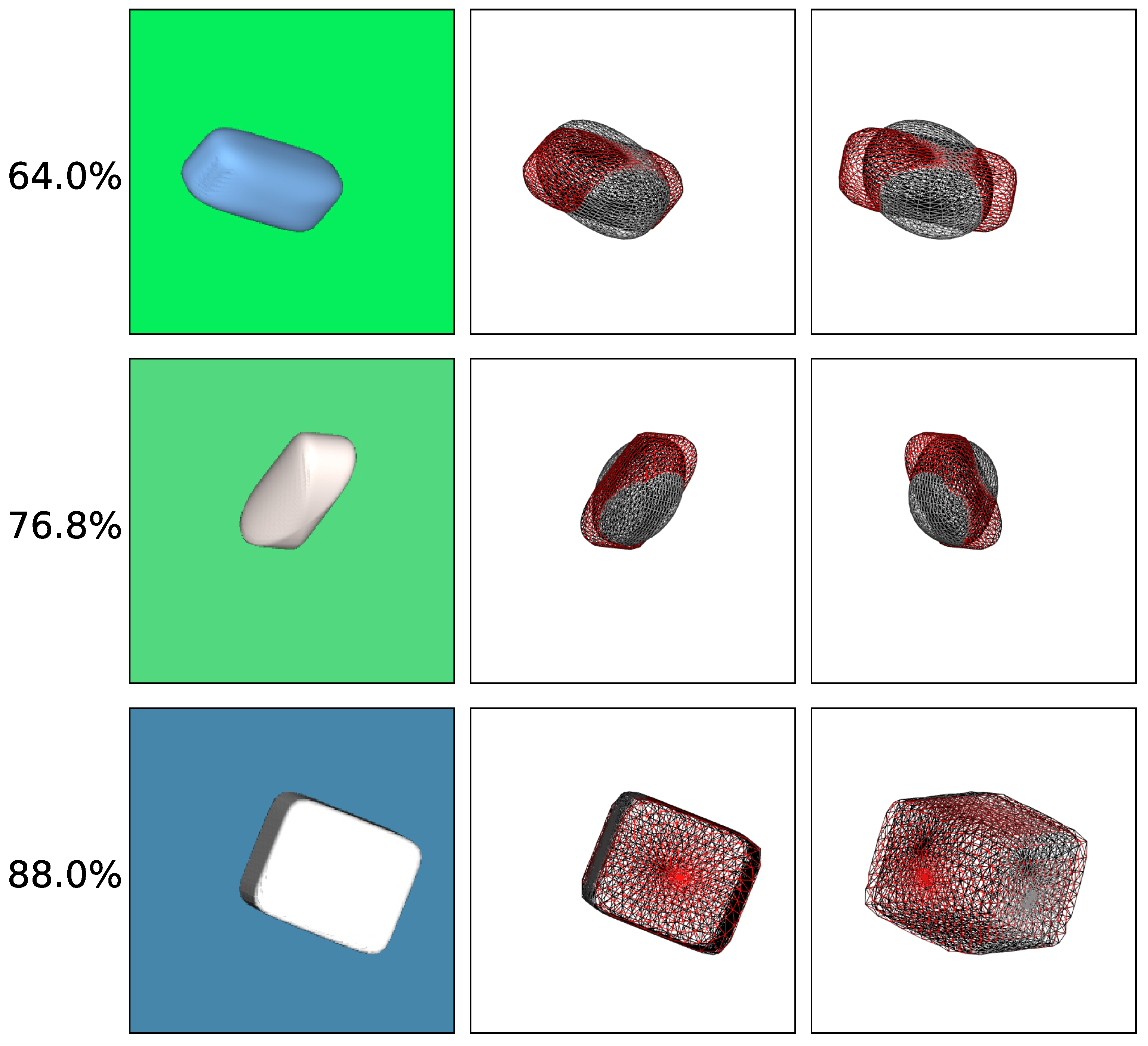
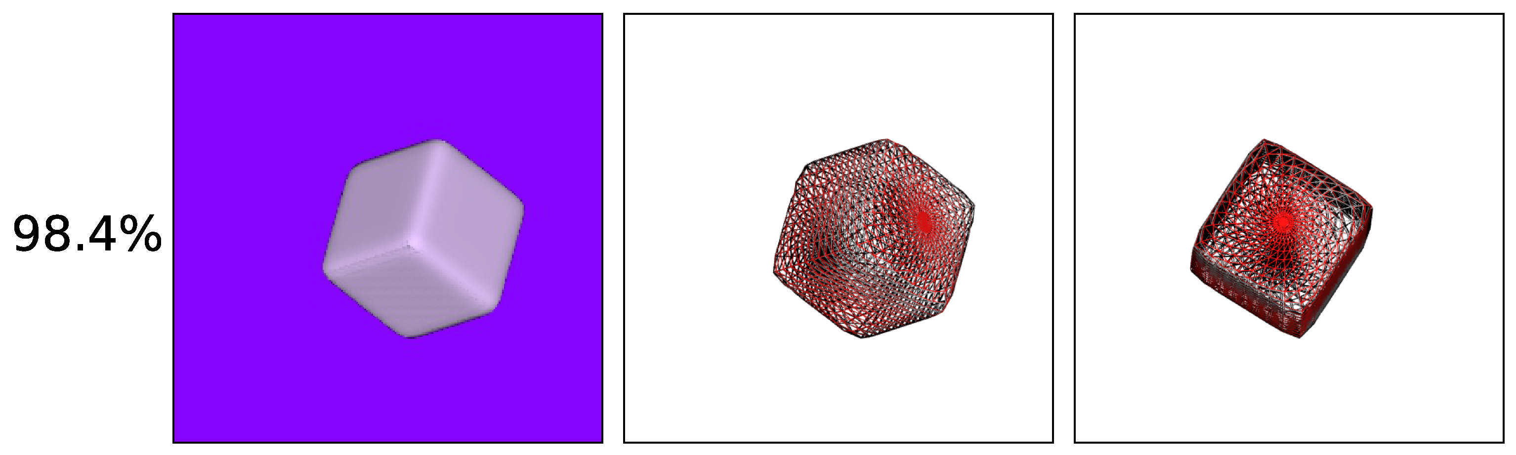
To better understand the accuracy of our predictions and the errors made, we also present qualitative results achieved with color images. We visualize the superquadric reconstructions of different accuracies in
Figure 9. To allow for easier visual comparison, we place both the ground truth superquadric wireframe (red) and the predicted superquadric wireframe (black) in the same scene. We then render the scene from two different points of view, the first being the same as when generating the original images, while the second is slightly moved. As expected, we observe considerable overlap between the wireframes of examples with high accuracy. In comparison, examples with low accuracy overlap quite poorly, which is especially noticeable when depicted from the alternative point of view.
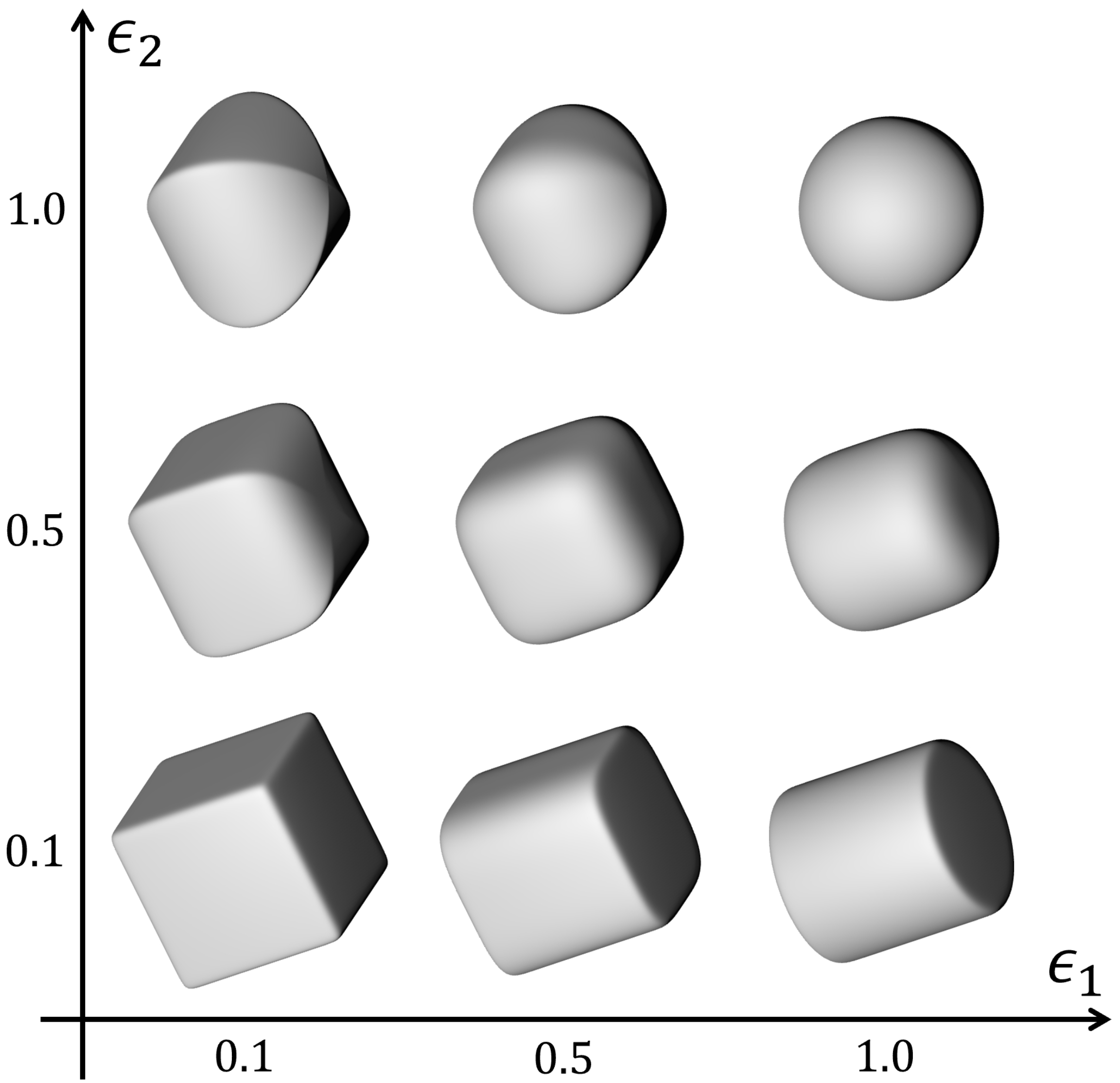
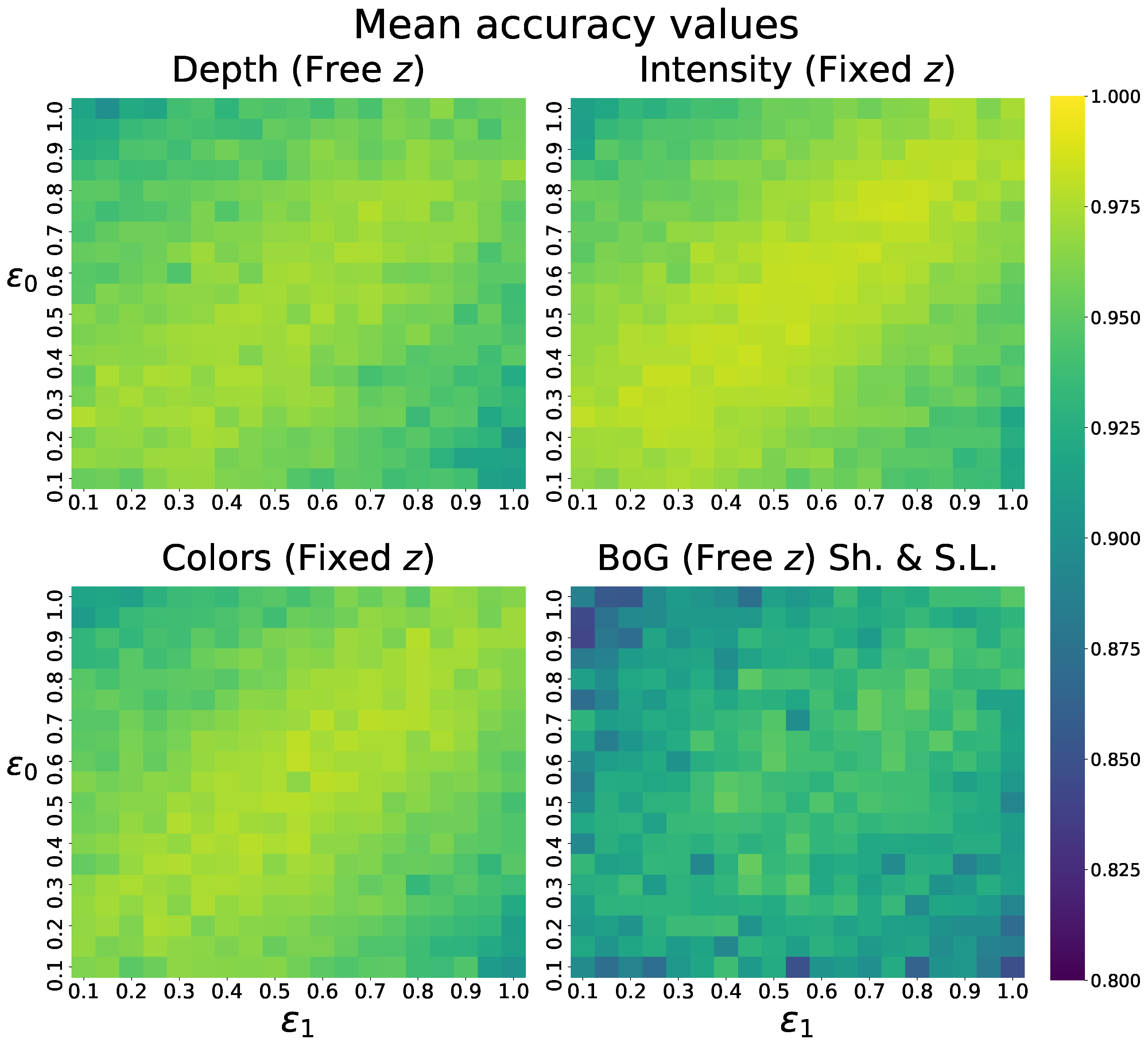
We also notice an interesting pattern in the qualitative results of this model and others, where the shapes of the superquadrics seem to be related to the obtained accuracy. To analyze this observation in a quantitative manner, we visualize the obtained mean IoU scores of multiple models across the ranges of both ground truth shape parameters
and
in
Figure 10.
From these heatmaps, it is clear that higher mean IoU accuracy is obtained along the diagonal when both shape parameters are fairly similar. Lower IoU accuracy is observed in corners where the two parameters are least similar. This means that our model more accurately predicts superquadrics, which are of symmetrical shapes, such as cubes and spheres, and less accurately predicts non-symmetrical shapes, such as cylinders. We believe that this occurs due to the ambiguity of the superquadric definition, discussed before, since symmetrical shapes allow for reordering of other parameters, without affecting the final superquadric. From this, we can simply conclude that non-symmetrical superquadrics are much more difficult to reconstruct than symmetrical ones, which should be taken into account in future research.
Throughout these experiments, we observed overall extremely positive results. The model based on the randomly colored dataset, with the
z position constraint, actually still outperforms the model based on depth images [
13]. Although the model performs slightly worse on the textured dataset, which is drastically more complex, the performance is still comparable. However, it should be noted that to allow for a more fair comparison, the aforementioned position constraint should first be addressed.
4.5.2. Solving the Fixed z Position Requirement
We have shown that our CNN predictor is capable of highly accurate superquadric reconstruction, under the condition that the z position in space is fixed. Without this undesirable requirement fulfilled, the accuracy of the reconstructions drops drastically.
To obtain promising reconstructions without additional constraints, we experimented with various possible solutions. In our first approach, we changed the perspective of the camera to an isometric view, prior to the rotation being applied to the superquadric. Unfortunately, this change simply spread the uncertainty across multiple parameters, since the same image could be captured with multiple variations of size and position. For example, the same image could be achieved with a larger object that is positioned further away from the camera.
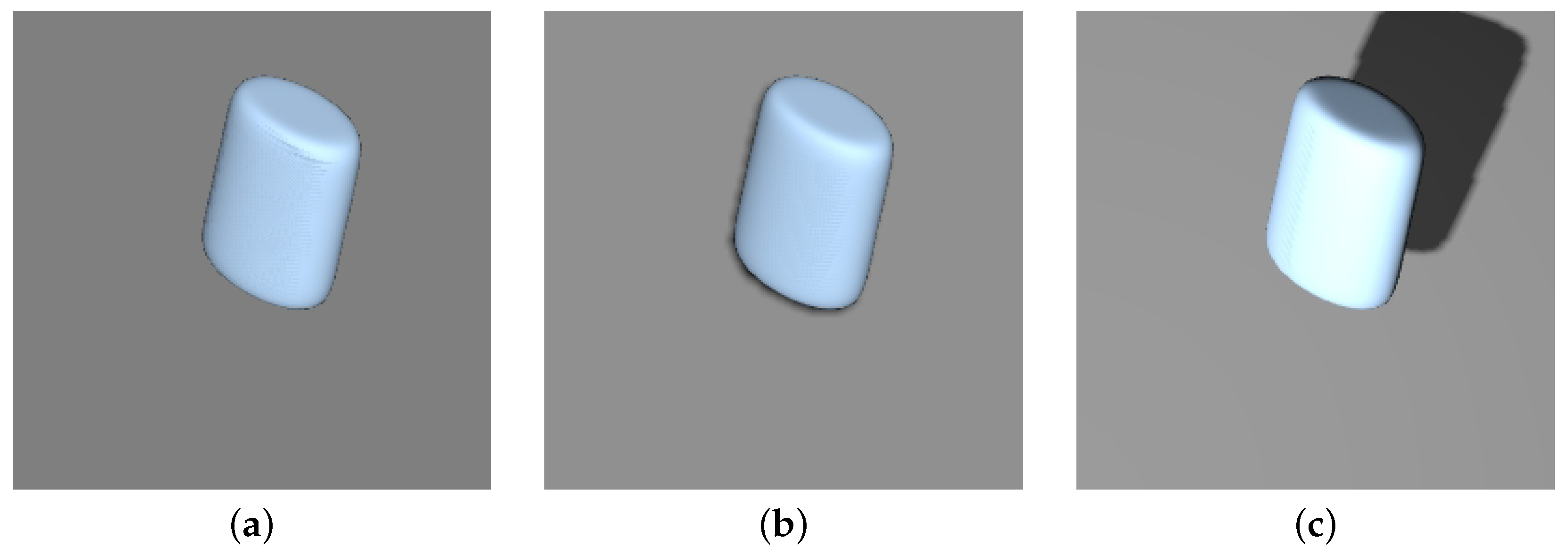
A more successful approach entailed enabling superquadrics to cast shadows on the background object. The added shadows are barely noticeable in the images, as seen in
Figure 11, due to the directional light source. In the dataset, the superquadrics are light blue and rendered in front of a gray background (referred to as Blue on Gray, or simply BoG), to allow for better contrast between the object, shadows, and background. This approach was inspired by various research studies [
16,
17], which showcased the importance of shadows for shape or size estimation. Our idea was that even these minimal shadows and their size differences could help with predicting the
z position parameter, alleviating the dependence on fixing this parameter.
Training and testing our CNN predictor on these images, we observed a drastic improvement in IoU scores. The
Blue on Gray (Free z) with Shadows model achieved a score of
in comparison with the results obtained on images without these alterations or the
Fixed z parameter (
), denoted in
Table 1, as
Blue on Gray (Free z). We can compare the performance of this approach with the original one, where the
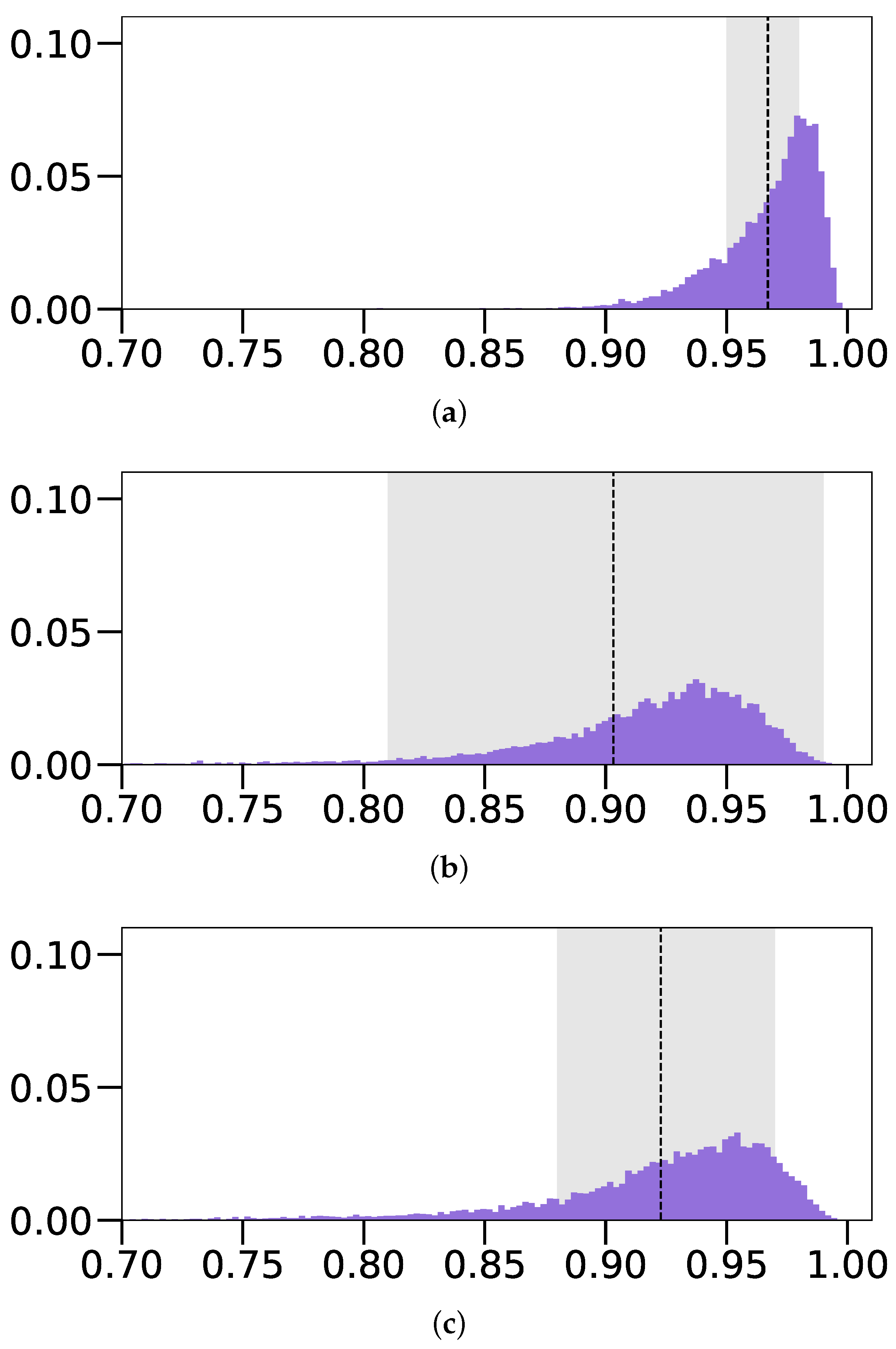
z parameter is fixed, via the IoU score distributions present in
Figure 12. The unrestricted approach with shadows (
Blue on Gray (Free z) with Sh.) displays a notable performance decrease in both the average IoU score and standard deviation, in comparison with the
Fixed z variant (
), denoted as
Blue on Gray (Fixed z). Observing the MAE scores of both models in
Table 1, we notice a drastic increase in position errors, due to the addition of the
z parameter, while size and shape errors remain fairly similar. Overall, these results reveal that we can bypass the requirement for the
Fixed z position parameter, at a modest cost of the performance, just by considering barely visible shadows.
In an attempt to further improve these reconstruction results, we added an additional spotlight source (S.L.) to the scene, as described in
Section 3.4, thus changing the position, size, and shape of the shadow cast by the superquadric. An example of the described alteration to the superquadric images can be seen in
Figure 11. Analyzing the results of the
Blue on Gray (Free z) with Sh. & S.L. model, we observe an average IoU increase of about
over the previous model without the spotlight, with the IoU scores being
. Interestingly, we notice substantially lower MAE values of the
x and
y position parameters, as well as a considerable decrease in the standard deviation for all position parameters. Inspecting the MAE distributions in
Figure 7, we can see that all distributions of the first BoG-based models without
z constraints (
Blue on Gray (Free z)) are heavily skewed, exhibiting rather unstable behavior. The MAE distributions of the second BoG-based model with shadows (
Blue on Gray (Free z) with Sh.) display drastic improvements; however, some of the distributions are still slightly skewed and not centered around an error of 0. In comparison, the final BoG-based model with the spotlight source (
Blue on Gray (Free z) with Sh. & S.L.) performs considerably better as all MAE distributions somewhat resemble Gaussian-like distributions. Despite their peaks not being as high as the ones obtained from other
Fixed z model variants, the distributions are at least centered around the 0 value.
Solving the
z position constraint also finally allows for a fair comparison between reconstruction from a single RGB image versus a single depth image [
13]. Comparing the results of the
Blue on Gray (Free z) with Sh. & S.L. model and the
Depth model [
13], we only note an accuracy difference of 0.035 in favor of the
Depth model. This shockingly small difference is impressive from our point of view, especially when considering the clear advantage that the latter approach has, in terms of available spatial information. The reason for the difference is also clearly evident when observing MAE values of the position parameters, where the largest difference is reported for the
z position parameter, as expected. In comparison, other parameters exhibit considerably smaller differences, especially the shape parameters.
From these results, we can conclude that more prominent shadows, obtained with an additional spotlight source, provide enough spatial information for highly successful reconstruction, without any position constraints. With this change to the artificial images, we are able to train substantially better performing predictors, which are even comparable to the model based on depth images [
13].
4.5.3. Comparison with the State-of-the-Art
With the next set of experiments, we compare our superquadric reconstruction method with one of the current state-of-the-art methods introduced by Paschalidou et al. [
10], whose work focuses on the reconstruction of complex 3D shapes with multiple superquadrics.
To obtain the required results for the experiments, we relied on the freely available source code (available at:
https://github.com/paschalidoud/superquadric_parsing, accessed on 8 December 2021), which accompanies the work by [
10]. To allow for a fair comparison of results, we limited the number of superquadrics recovered by the aforementioned method to one. Since this change makes several parts of their method redundant, we also ignored the parsimony loss, responsible for scene sparsity. This model was originally used with voxel form data, such as objects from the ShapeNet dataset, but it also works with other forms of data. Unfortunately, we encountered several problems with convergence when using RGB images, resulting in a rather bad overall performance. Thus, we chose to use the voxel form representation of data, as originally intended by the authors [
10]. This decision makes our comparison slightly more difficult since the difference between RGB images (used by our method) and the voxel representation is rather drastic. Most importantly, the latter provides significantly more spatial information, due to our images being limited to a single point of view, which results in the occlusion of some parts of the superquadric. Furthermore, RGB images lack depth information, which was already discussed in previous sections. Due to these differences, we hypothesize that the method by Paschalidou et al. [
10] should outperform our method.
To train their model on our synthetic superquadric dataset, we represent each superquadric scene in our datasets with a voxel grid of size
, as defined in [
10]. The method by Paschalidou et al. [
10] also provides users with various learning settings, which we experimented with to obtain the final model. We used a similar learning procedure to the one presented in previous sections and trained the model until convergence.
We report the average and standard deviation values of both methods on two datasets and their subsets in
Table 2—these datasets being the intensity dataset with the
Fixed z parameter and the Blue on Gray (BoG) dataset with the
Free z parameter, shadows, and a spotlight. We also experimented with subsets of the datasets because the initial experiments of Paschalidou et al. [
10] were performed on superquadrics with shape parameters between 0.4 and 1.5, while shape parameters in our dataset ranged from 0.1 to 1.0. To ensure a fair comparison, we trained and tested the two methods first on the entirety of each dataset and then on a subset of the dataset, whose parameters lie between 0.4 and 1.0 as a compromise between the ranges of both papers. This subset included 4417 images of the initial 10,000 image test set.
For the first experiment, we used the dataset based on intensity images of superquadrics with the
Fixed z position parameter (
Intensity (Fixed z)). The results of this experiment, reported in
Table 2, are rather clear. On the entire dataset, our method achieves considerably better reconstruction performance than the method by Paschalidou et al. [
10], with the difference in terms of average IoU scores being 0.168. The latter method also performs worse in terms of standard deviation. Nevertheless, using the entire dataset favors our method, due to the shape parameter range, so we also consider results on the subset of the dataset. The method by Paschalidou et al. [
10] displays a larger improvement in IoU scores than our method on the given subset. However, the performance differences between the methods remain quite large (0.159 on average). Interestingly, the method by Paschalidou et al. does not improve in terms of standard deviation, while ours does.
Because we are aware of the effects that such a configuration, with
Fixed z position parameters, can have on the final reconstruction results, we also trained and tested the two methods on a dataset without this constraint. For this, we used the Blue on Gray dataset with shadows and a spotlight source (
BoG (Free z) with Sh. & S.L.), in order to provide our model with enough spatial information via shadow-based cues, as discussed in
Section 4.5.2. For the method by Paschalidou et al., we again used the voxel representation of superquadric scenes, which provided plenty of spatial information about the position in space. Thus, the method should not have reconstruction issues, despite dealing with the slightly more complex task of properly predicting an additional position parameter.
Despite the clear advantage that the method by Paschalidou et al. has in terms of available information, we observe that our method still performs notably better, both on the entire dataset and its subset. Nevertheless, the method by Paschalidou et al. was not noticeably affected by the lack of the z position parameter restriction. On average, the IoU score was reduced by 0.024 and 0.026 for the entire dataset and its subset, respectively. In comparison, the performance of our method was impacted heavily by this change, despite the addition of shadows. This can be seen in the decrease of the average IoU scores by 0.043 and 0.040, respectively, alongside major increases in standard deviation values. Overall, we observe that the difference in model performance is slightly smaller on the dataset without the z position parameter restriction. However, the difference is still clearly evident.
Nevertheless, it should also be taken into consideration that the method by Paschalidou et al. [
10] was not explicitly designed for the reconstruction of simple objects with a single superquadric, but rather for reconstruction of complex objects with multiple superquadrics. Despite this, the above analysis still showcases the power of our reconstruction method among current state-of-the-art approaches on the task of reconstructing simple objects. In turn, it also shows the potential of using our method for future practical approaches, such as robot gras**.
4.5.4. Performance of Different Backbone Architectures
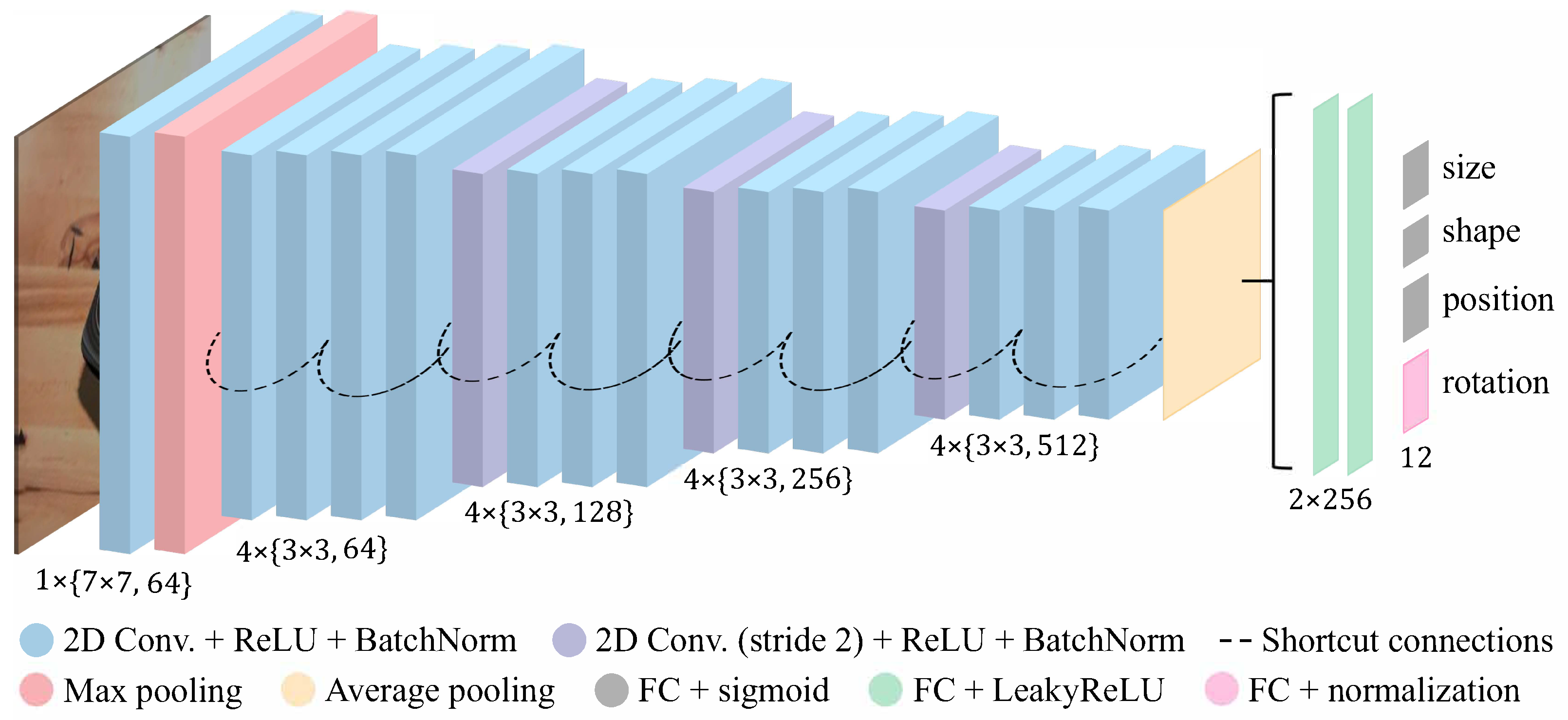
To evaluate the choice of backbone architectures, used for our CNN predictor, we compare the performance of the predictor using two different backbone networks, namely the ResNet-18 [
42] and the Inception-V3 network [
50], in terms of reconstruction accuracy. Similar to previous experiments, we evaluated the performance of both variants on two datasets,
Intensity (Fixed z) and
Blue on Gray (Free z) with Sh. & S.L., whose images differ drastically in complexity. To allow for a fair comparison, we trained both variants of the CNN predictor under identical training conditions, following the description in
Section 4.4, and trained and tested them on the same datasets. We report the average IoU score and standard deviation values achieved by the two different backbone architectures on the two datasets in
Table 3.
For the first experiment on intensity images with a Fixed z position parameter (Intensity (Fixed z)), the model with the ResNet-18 backbone architecture clearly outperforms the Inception-V3 variant in terms of reconstruction accuracy, with the difference of average IoU scores being 0.360. Furthermore, the ResNet-18 variant also achieves a drastically lower standard deviation (only 0.022), meaning that this model performs more consistently across a wide range of superquadrics. In comparison, the standard deviation of the Inception-V3 variant is incredibly high (0.146), showcasing that the predictions across the entire test dataset are clearly not as stable, despite being rather successful on average.
In more complex images, namely the Blue on Gray (Free z) with Sh. & S.L. dataset, we observe that the ResNet-18 variant still outperforms the Inception-V3-based one. However, it should be noted that the performance of the ResNet-18 variant decreases considerably, by 0.043 on average, while the performance difference of the Inception-V3 variant is not as drastic, only 0.010 on average. More interestingly, while the standard deviation of the ResNet-18 variant increases with more complex images, as expected, it decreases for the Inception-V3 variant. However, the ResNet-18 variant still outperforms the latter.
Despite having significantly more trainable parameters (24 million), the Inception-V3 network still performs considerably worse, overall, than the ResNet-18 variant, with only 11 million trainable parameters. We speculate that this might be due to the over-complication of the map** between the input and output of the Inception-V3 variant. This is solved by skip connections in the ResNet-18 network, which allow for simple map**s and also address the vanishing gradient problem during training. This in turn also explains why the difference in performance between the two models is noticeably lower on the more complex dataset, as the strong shadows in the images necessitate a more complex map** and a larger network. Furthermore, since the network is wider and uses multiple kernels of various sizes within the same layer, it should be more suitable for gathering both global and local features from more complex images. Nevertheless, considering all the aforementioned observations, we conclude that for the task at hand the ResNet-18 backbone architecture is the most appropriate, due to its high reconstruction accuracy and efficient training. However, the inclusion of the wider Inception-V3 backbone could prove useful in future research, especially with the transition to larger and more complex images.
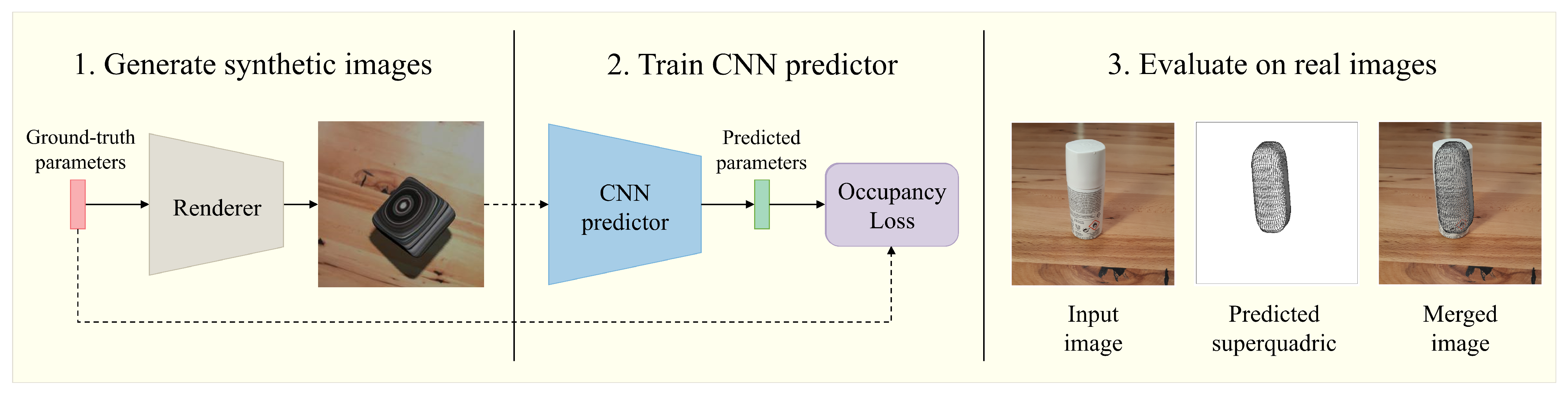
4.5.5. Performance on Real Images
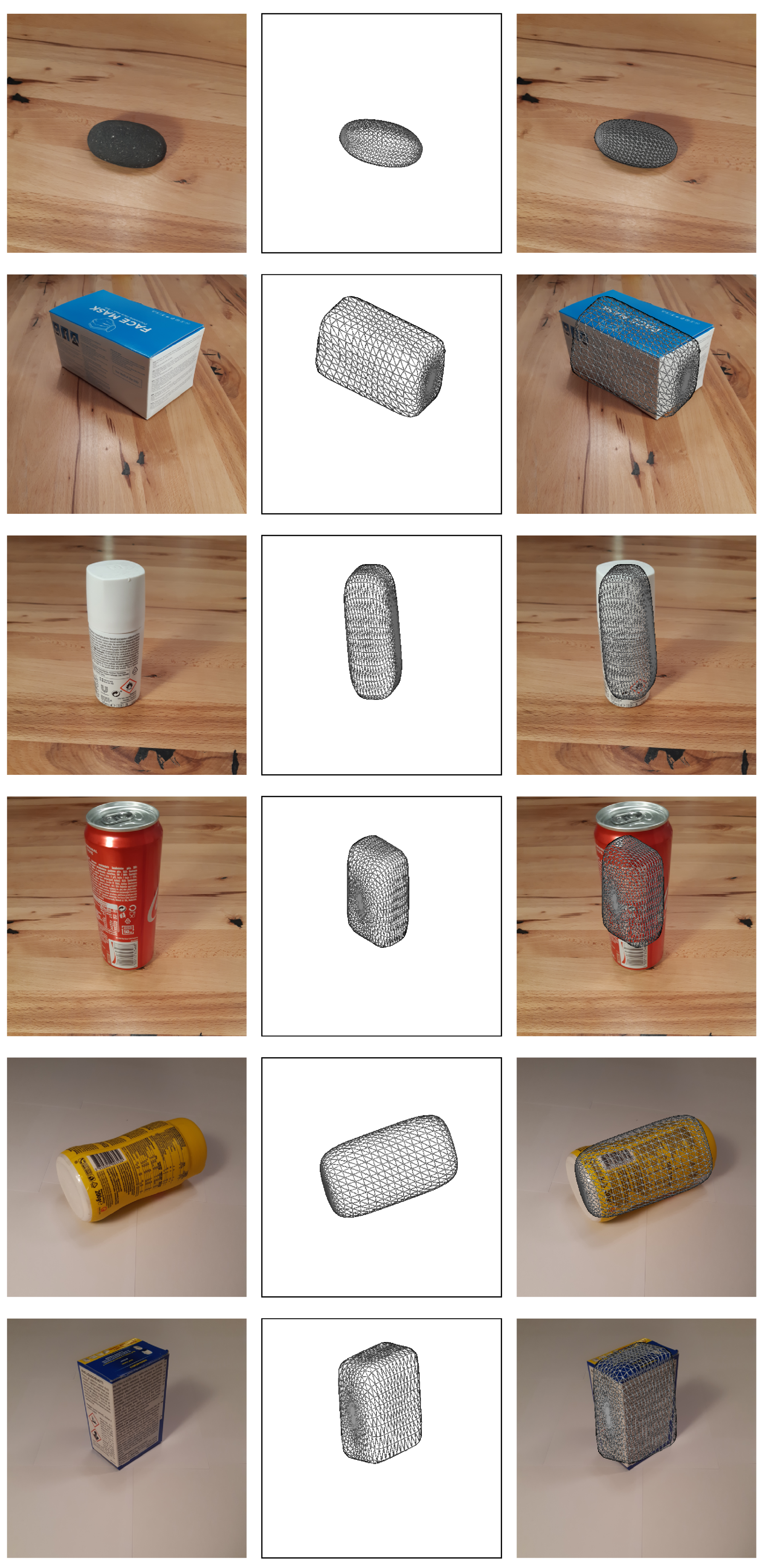
Finally, we analyzed the performance of our reconstruction method on real-world data. To do this, we trained the CNN predictor on synthetic images and tested its performance on real images. First, we captured images of various objects with a phone camera, on a wooden and a white background, and then resized the images to fit the input of our CNN predictors. Examples of the real images used are present in the first column of
Figure 13.
To recover superquadrics from these real images, we first tested all trained models discussed above. However, we observed little to no success, as was expected, due to immense differences between the training and testing data. For example, real images included significantly more detailed textures of objects and backgrounds, in addition to the slight difference in projection style. Furthermore, most objects cannot be perfectly described by a single superquadric, due to their more complex shapes. Thus, we decided to construct a new training dataset that would mimic the captured images. To obtain more realistic images, we replaced the vast variety of textured backgrounds with real wooden textures, captured in the same location as the real images. To ensure some variety in training samples, we used 5 different images of the wooden texture. For each generated image, we randomly selected one texture image for the background and then randomly rotated it. In addition, we allowed the superquadric to cast shadows on the background and used the spotlight source. For this task, we constructed two datasets, with one following the Fixed z position constraint and another without this constraint, to explore which configuration performed better with real images.
Having trained the two new models, denoted in
Table 1 as
Textured on Wood (Fixed z) with Sh. & S.L. and
Textured on Wood (Free z) with Sh. & S.L., we first tested them in a similar fashion as before on the test datasets. We observed fairly high IoU scores for the above-mentioned
Fixed z variant (
), which were slightly worse, both in terms of average and standard deviation, than the scores of the previous
Textured (
Fixed z) model (
). Interestingly, as can be seen in
Table 1, the new model (
Textured on Wood (Fixed z) with Sh. & S.L.) achieved worse MAE scores for the size and shape parameters, but better results for the position parameters, which most likely contributed to the differences in IoU scores. This reveals that the addition of shadows in the scene alongside more realistic backgrounds can negatively impact the performance of our simple CNN predictor, despite being necessary to approach realistic images. In comparison, we observed a considerable drop in performance with the
Free z variant (last row in
Table 1), which achieved an IoU score of
. However, it should be noted that it did predict all parameters, showcasing that relying on the
Fixed z requirement is not necessary. Unfortunately, this model (
Textured on Wood (Free z) with Sh. & S.L.) did not perform as well as the model in the previous section (
Blue on Gray (Free z) with Sh. & S.L.), despite the main difference only being the textures. We observed that these textures drastically affected the shading and shadows of certain superquadrics. This might be the reason for the performance difference since such information is crucial for the CNN predictor when faced with the
Free z configuration. We believe this is the reason why the majority of
Fixed and
Free z models trained on uniformly colored images, discussed in previous sections, performed considerably better than their
Textured on Wood counterparts.
Finally, we tested both
Textured on Wood models on the gathered real images and noted that the
Free z configuration performed very poorly. In comparison, the model trained on the
Fixed z image configuration performed fairly well, at least based on qualitative results, displayed in
Figure 13. Here, the first column depicts the original image and the second shows the wireframe of the predicted superquadric. By inspecting the last column, which overlaps the wireframe over the input image, we observe that in quite a few of the examples the wireframe fits the captured object quite nicely. Interestingly, being trained on synthetic images with wooden backgrounds, the model (
Textured on Wood (Fixed z) with Sh. & S.L.) also performs incredibly well on real images with white backgrounds. In our experiments, we observe that, despite different backgrounds, the model subjectively outperforms all others, even those trained on images with uniformly colored backgrounds. This might be caused by the evident shading differences between realistic white backgrounds and artificially colored ones. Despite numerous successful reconstructions, there still exist quite a few suboptimal reconstruction examples for both background configurations. These examples showcase that the model remains rather unpredictable in real images. This could be due to slightly more complex shapes of real objects that superquadrics cannot recreate. Another possible reason could be the slight change in image projection since the model was trained on images rendered in orthographic projection, while real images were captured in perspective projection.
Results of this experiment show that our approach is able to generalize well from artificial training data to real-world data, and is able to successfully reconstruct various simple objects, despite clear differences between the training and testing data. Based on our testing, we believe that the model could also generalize to different real-world scenes if the training images include even more background variety. Overall, these real-world experiments showcase the potential of our approach for future practical applications, for example, for robots gras** unknown objects based on a single RGB image.


