4.3. Power Cable Fault is Processed by the ACCLN Method
In this section we apply the ACCLN method to deal with power cable fault types. The data in [
16] is used to recognize the power cable fault types. There are three kinds of fault types in [
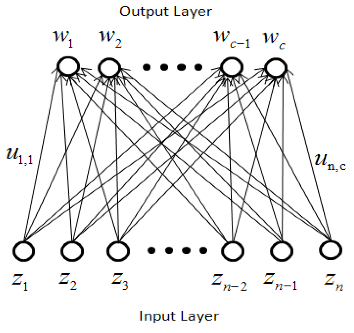
16], interphase short circuit, three phase short circuit, and normal condition, respectively. A total of 54 sample data are used in the experiment. The ACCLN consists of a neuron array 54 × 1 in the input layer and three neuron nodes in the output layer. The transient state
and the internal state
are 54 × 3 array. Each testing point of phase entropy and amplitude entropy are composed of an input vector, and normalized in the input layer. The phase entropy and amplitude entropy are normalized as follow. For example, for each phase entropy and amplitude entropy, the normalized value is shown as Equations (20) and (21):
and an input vector
is shown:
Where
indicates the
i-th phase entropy,
and
is the minima and maxima of the 54 phase values, respectively.
is the
i-th normalized phase value. The process of normalizing amplitude entropy is the same as phase entropy.
is the
i-th input vector, composing the normalized phase value
and the normalized amplitude value
.
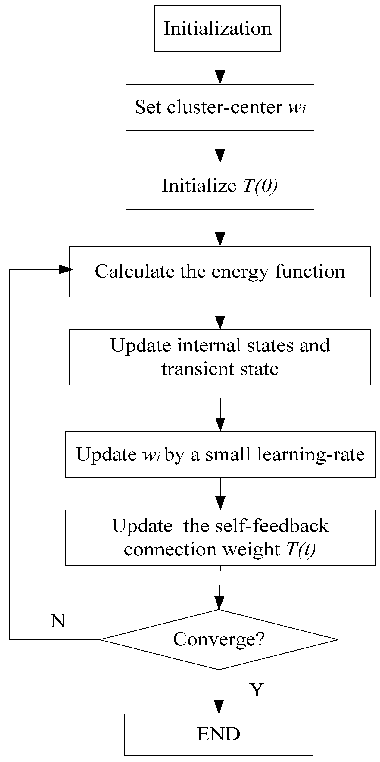
The flow chart of ACCLN algorithm is shown in
Figure 9. The step of ACCLN algorithm for power cable fault classification is shown as follow:
Step 1: Preprocess the input phase entropy and amplitude entropy for each test point using Equations (20–22).
Step 2: Set the cluster-center
(j=1,2,3...) randomly for interphase short circuit, three phase short circuit, and normal condition.
Step 3: Initialize self-feedback connection
, internal states and transient state for all interconnection strengths.
Step 4: Calculate the energy function (14).
Step 5: Update internal states and transient state for all interconnection strengths using Equations (15) and (16).
Step 6: Update the cluster-centers by a small learning-rate parameter using Equations (17) and (19).
Step 7: Decrease the self-feedback connection weight
using Equation (18).
Step 8: If the network does not converge then goes to Step 4; otherwise stop.
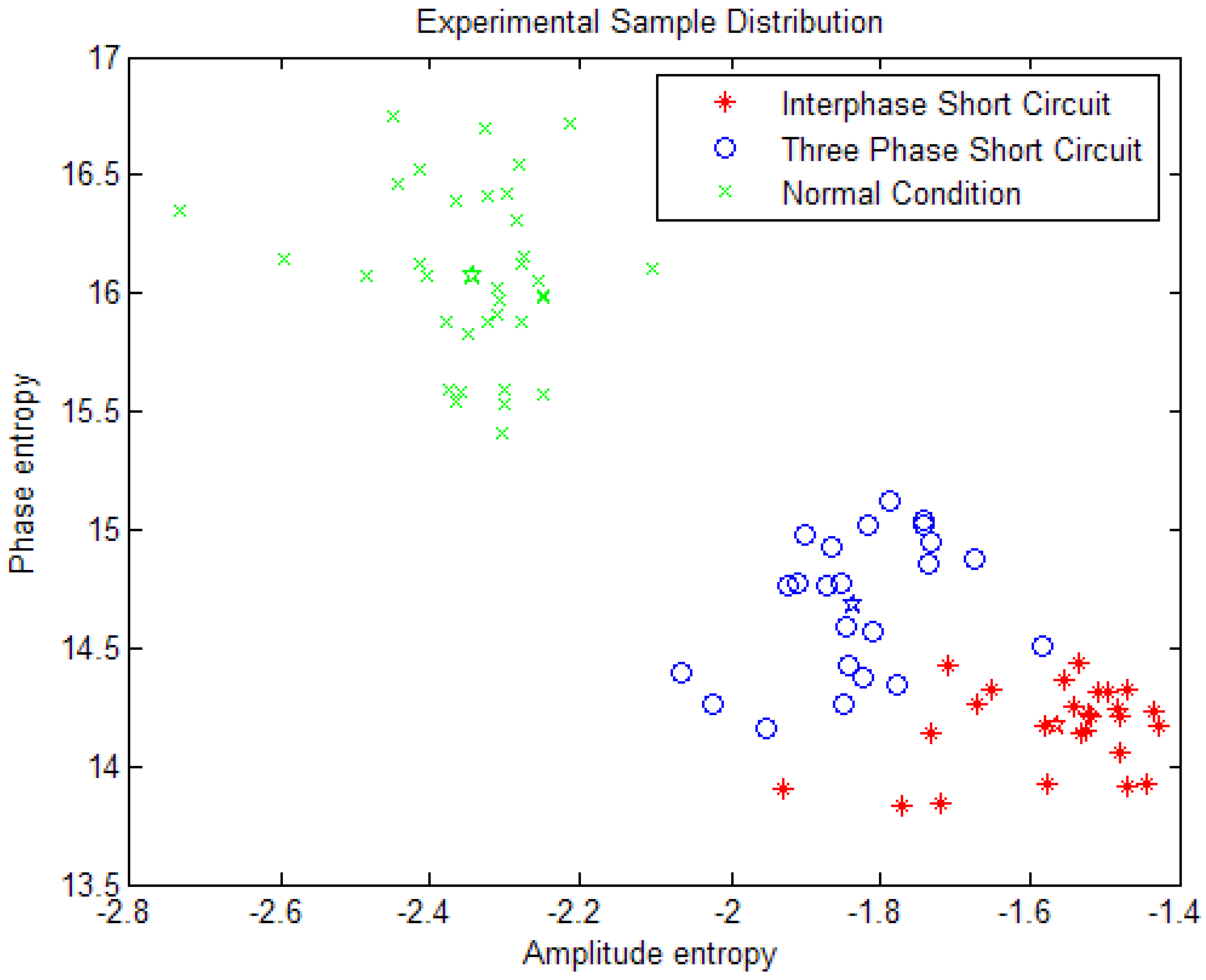
Figure 10 shows the experimental sample data distribution. There are 6 category data, interphase short circuit of training data and test data, three phase short circuit of training data and test data, normal condition of training data and test data, respectively. The recognition accuracy was 87.0% with the SVM method and 90.7% with the IPSO-SVM method in [
16].
Figure 9.
Flow chart of annealed chaotic competitive neural network (ACCLN).
Figure 9.
Flow chart of annealed chaotic competitive neural network (ACCLN).
Figure 10.
Experimental sample data distribution. X axis indicates amplitude entropy; Y axis indicates phase entropy.
Figure 10.
Experimental sample data distribution. X axis indicates amplitude entropy; Y axis indicates phase entropy.
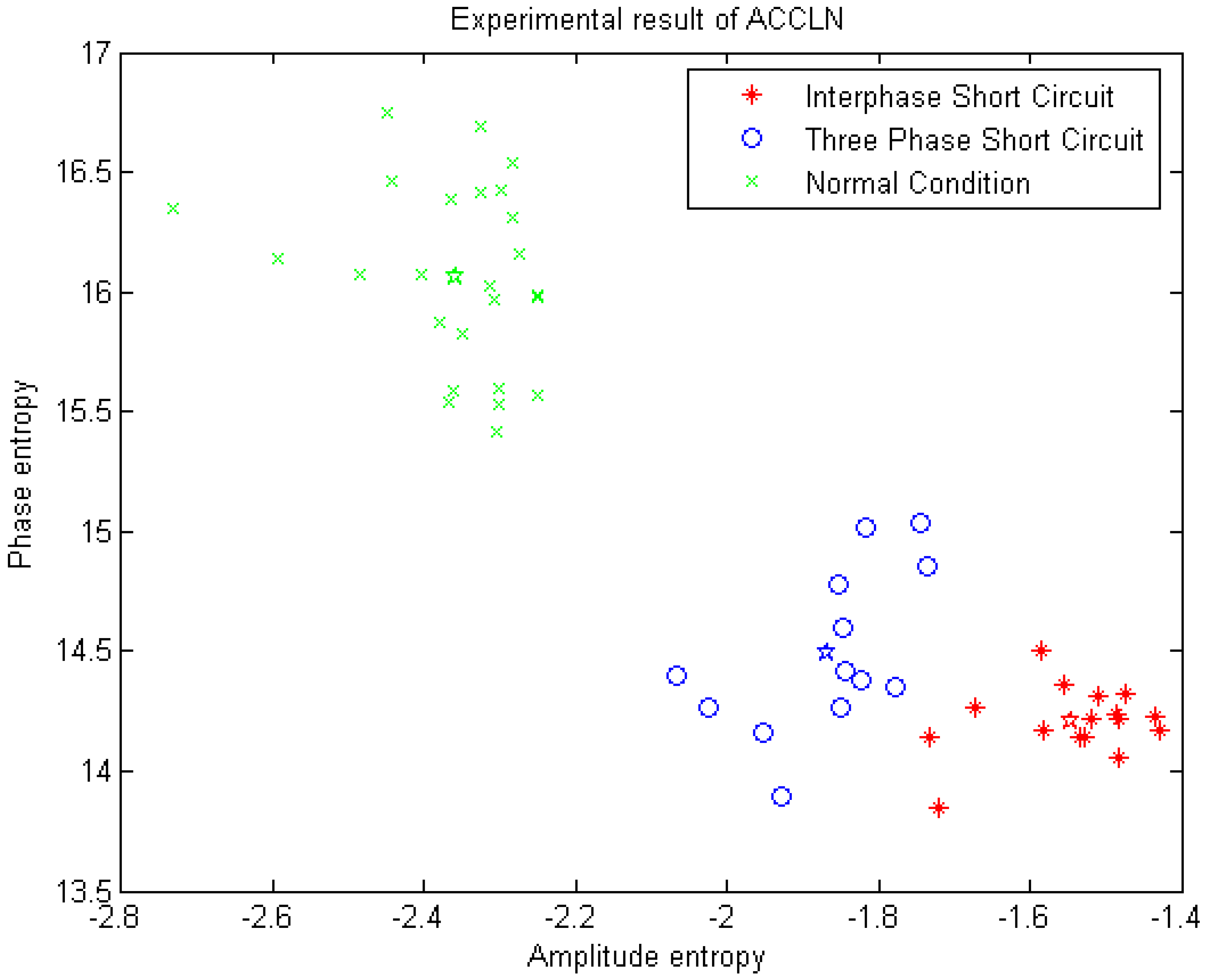
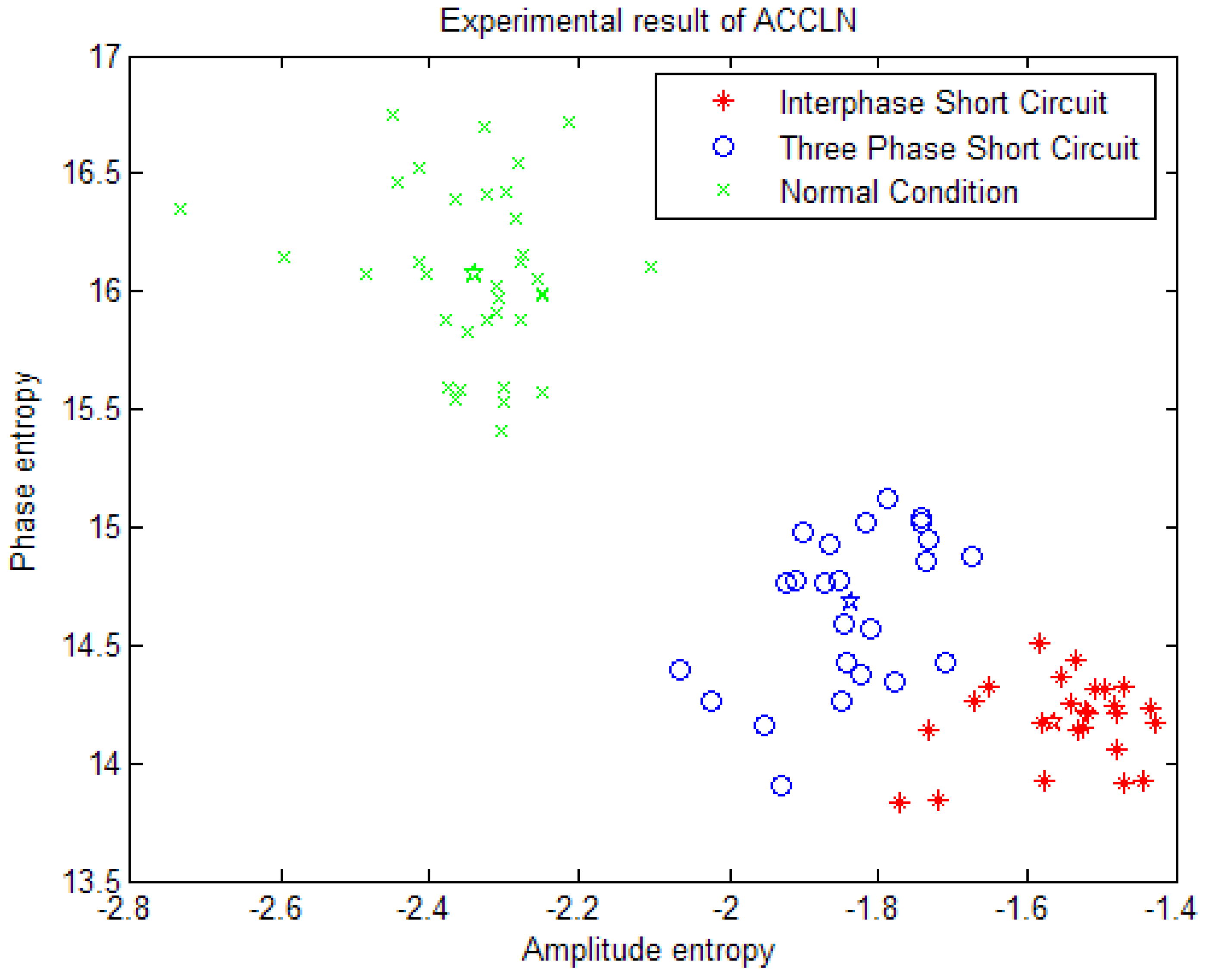
Figure 11 shows the experimental result of ACCLN. There are 54 sample data. Those samples are divided into three classifications. The green “
![Algorithms 07 00492 i001]()
” indicates normal condition of power cable, 25 samples. The blue “
![Algorithms 07 00492 i002]()
” indicates the power cable of three-phase short circuit, 13 samples. The red “
![Algorithms 07 00492 i003]()
” indicates the power cable of interphase short fault, 16 samples. The different colors “☆” corresponds to each cluster-center.
Figure 11.
Experimental result of ACCLN. X axis indicates amplitude entropy; Y axis indicates phase entropy.
Figure 11.
Experimental result of ACCLN. X axis indicates amplitude entropy; Y axis indicates phase entropy.
Table 2 shows the recognition accuracy of SVM, IPSO-SVM, and ACCLN methods. The recognition accuracy of ACCLN, IPSO-SVM and SVM is 96.2%, 90.7%, 87.0%, respectively. The training times are 0.032, 0.0523, 0.0575, respectively. The performance of the power cable fault recognition of ACCLN method is better than SVM and the IPSO-SVM method.
Table 2.
Recognition accuracy of SVM, IPSO-SVM and ACCLN.
Table 2.
Recognition accuracy of SVM, IPSO-SVM and ACCLN.
| Algorithm | Recognition Accuracy | Training Time |
|---|
| ACCLN | 96.2% | 0.032 |
| IPSO-SVM | 90.7% | 0.0523 |
| SVM | 87.0% | 0.0575 |
In order to test the effectiveness of the proposed method, each group of dataset add 10 test samples, 30 test samples are added on the basis of original samples. So there are 84 test samples in experiment.
Figure 12 shows 84 sample distributions.
Figure 13 shows the result of ACCLN method. The recognition accuracy of ACCLN is 96.4%.
Figure 12.
Experimental sample data distribution (84 samples); X axis indicates amplitude entropy; Y axis indicates phase entropy.
Figure 12.
Experimental sample data distribution (84 samples); X axis indicates amplitude entropy; Y axis indicates phase entropy.
Figure 13.
Experimental result of ACCLN (84 samples). X axis indicates amplitude entropy; Y axis indicates phase entropy.
Figure 13.
Experimental result of ACCLN (84 samples). X axis indicates amplitude entropy; Y axis indicates phase entropy.


 ” indicates normal condition of power cable, 25 samples. The blue “
  ” indicates the power cable of three-phase short circuit, 13 samples. The red “
  ” indicates the power cable of interphase short fault, 16 samples. The different colors “☆” corresponds to each cluster-center.

