Communication

Evaluation of Early Bark Beetle Infestation Localization by Drone-Based Monoterpene Detection

1
Department of Forest Work Science and Engineering, Georg August University Göttingen, Büsgenweg 4, 37077 Göttingen, Germany
2
Chair of Remote Sensing and Landscape Information Systems, Albert-Ludwig-University Freiburg, Tennenbacherstr. 4, 79106 Freiburg, Germany
3
Chair of Forest Utilization, University of Applied Forest Science Rottenburg, Schadenweilerhof, 72108 Rottenburg, Germany
*
Author to whom correspondence should be addressed.
Forests 2021, 12(2), 228; https://doi.org/10.3390/f12020228
Submission received: 15 January 2021 / Revised: 5 February 2021 / Accepted: 11 February 2021 / Published: 16 February 2021

Abstract

:
The project PROTECTFOREST deals with improvements in early bark beetle (e.g., Ips typographus and Pityogenes chalcographus) detection to allow for fast and effective response to initial infestation. The removal of trees in the early infestation stage can prohibit bark beetle population gradation and successive timber price decrease. A semiconductor gas sensor array was tested in the lab and attached to a drone under artificial and real-life field conditions. The sensor array was able to differentiate between α-pinene amounts and between different temperatures under lab conditions. In the field, the sensor responded to a strong artificial α-pinene source. The real-life field trial above a spruce forest showed preliminary results, as technical and environmental conditions compromised a proof of principle. Further research will evaluate the detection rate of infested trees for the new proposed sensor concept.

1. Introduction

Climate change and the corresponding temperature increase have an impact on the stability of forest ecosystems, especially on the distribution and activity of xylophagous beetles [1,2]. The economic effect of a higher xylophagous beetle activity was quantified for Canada, with an average annual loss of 1274 million dollars of the net present value between 2009 and 2054 [3]. In the USA, the annual loss was 1500 million dollars between 1971 and 2000 (equivalent to 41% of total annual loss including fire, hurricane, tornado, ice, invasive species, landslides, and drought) [4]. In Germany, infestation from the last three years (2018–2020) led to wood loss of 178 mio m3 [5], which is 4.9% of the wood stock calculated by the national forest inventory in 2012 [6].
The bark beetles Ips typographus and Pityogenes chalcographus show very high fertility in hot and dry seasons [2,7]. They can have up to four generations per year at an optimal temperature of 30 °C [8]. Detecting such a pest outbreak between four months and one year after the initial infestation, e.g., by alternating crown color [9], is far too late, as the bark beetle population multiplies by a factor of approximately 203–1003 per female individuum [8,10,11,12]. It was reported that the detection of beetle infestation at a late stage within the spectral range of 450–890 nm was possible with a prediction efficiency of 64%. This approach is very sensitive to interactions with direct and scattered sunlight [13]. Comparable results were presented for the utilization of a hyperspectral camera [14]. This is a limited approach for pest control of aggressive species, e.g., Ips typographus, because early detection of green stage infestation is needed to prevent a gradation. Detecting trees in the red stage of infestation at low detection rates cannot prevent a gradation, though it could indicate larger areas with high infestation risk. Another approach is the utilization of satellite data for infestation extrapolation based on the easily identifiable grey infestation stage [15]. Although early detection methods are necessary in order to reduce timber losses caused by frequent bark beetle gradations, holistic approaches can allow a prediction system to narrow down the possible areas of infestation to optimize the search for green stage infestation.
Monoterpenes and especially α-pinene are considered to have an impact on global air quality [16], with forests as a major emission source [16,17,18]. A model study of Guenther et al. estimated the annual global forest volatile organic compound (VOC) flux at 1150 Tg C, with a share of 11% monoterpenes. A study by Berg et al. modeled the bark beetle attack with a low impact on overall forest emissions, although the emission impact of bark beetles on the overall tree mortality emissions was very high [19]. Monoterpene emissions differed between forest plant species [17]. In healthy conifer trees, the monoterpene emission is a function of the temperature-dependent vapor pressure that can be explained by the Clausius Clapeyron equation [20,21,22]. α-pinene was found to be emitted in a diurnal cycle in forests [16]. This shows that, in healthy plants, monoterpenes are emitted passively through the stomata.
Monoterpenes belong to the group of plant VOCs that increase in concentration after plant damage (inducible VOCs) [23] or drought stress [22,24]. Coniferous trees can emit increasing amounts of monoterpenes after an attack of xylophagous beetles by induced host defense mechanisms [25,26,27,28]. These emissions are caused by leaking resin from physically damaged resin channels below the bark and by the general stress response of the tree. The resin consists of resin acids and monoterpenes. The monoterpenes are a nonpolar solvent for resin acids that decreases their viscosity and enables their flow into the bark hole. There, the solvent evaporates, the resin acids start to polymerize, and the hole closes. This mechanism enables the tree to defend itself by “resinating” the beetle out of its bore hole and by successively closing the bore hole. The general stress response comprises the increase in monoterpene cyclase levels after damage to a 5 to 15 times higher level. Therefore, trees produce monoterpenes after physical damage to restore their host defense capability [29] and to passively emit more monoterpenes through the stomata [20,21,22]. The major resin components in economically relevant coniferous trees in boreal and temperate forests are monoterpenes and, among the group of monoterpenes, especially α-pinene [11,26,27,28,30]. This compound is an attractant for bark beetles as well [11,31]. It is usually emitted by infested trees in the early or “green” stage of the pest attack [25,27]. However, an increased emission in the yellow stage was reported as well [26]. Drought stress also has a strong impact on α-pinene emission. The effect of draught is discussed controversially in the literature, as both increases and decreases in emission rates were detected [22,24]. Table 1 shows an overview on the literature that quantified emissions from infested forest trees or forest trees under drought stress.
Bark beetle pheromones are produced and dispersed by the beetles and can be a cue for individuals of the same species to gather or disperse according to the nutritional state of the host plant [12,31,32]. Interspecific pheromone interactions among bark beetle species were reported as well [33]. The chemical ecology of bark beetles was reviewed by Blomquist et al., by Tittinger and Bloquist [31,34], and by earlier sources [35,36,37]. The concentration of bark beetle pheromones is several orders of magnitude lower than the concentration of α-pinene in forests [38]. The beetles are comprised of a biological detection system that is based on odorant-binding proteins (OBPs). The OBPs allow the selective binding of VOCs and their transportation to neurons in the beetles antennae for information processing [39,40,41]. Binding sites of OBPs and especially of the subgroup pheromone-binding proteins (PBPs) can be highly selective and low VOC concentrations can elicit a neuronal response [41].
Semiconductor metal-oxide gas sensors are feasible detectors for volatile organic compound (VOCs) classes in air, like monoterpenes. A semiconductor surface, e.g., tungsten oxide, changes its conductance when it is heated. At a constant and high temperature, e.g., 275 °C, the oxidation state of the oxygen atoms in the molecular tungsten oxide grid determines the conductance. When VOCs interact with the heated semiconductor tungsten oxide surface, they are thermally oxidized. The oxygen atoms in the tungsten oxide grid can also change their oxidation state due to the electron exchange in the thermally induced conversion of the VOCs. This electron exchange can oxidize or reduce the oxygen in the metal oxide. This leads to a conductance decrease in the metal oxide. The intensity of this decrease is usually not VOC-specific but VOC class-specific [42]. The VOC class selectivity can be improved by using several metal oxide sensors that exhibit different reaction intensities, thereby creating a VOC class-specific signal pattern. Earlier studies used a gas sensor below a quadcopter in the rotor down winds to obtain signals while flying through a large smoke plume [43]. This study investigates the monoterpene detection performance of an quadcopter semiconductor gas sensor system using α-pinene as a model compound. The sensor setup is based on three semiconductor gas sensors with different surface properties and a sampling option to sample the undisturbed air outside the rotor down winds.

2. Materials and Methods

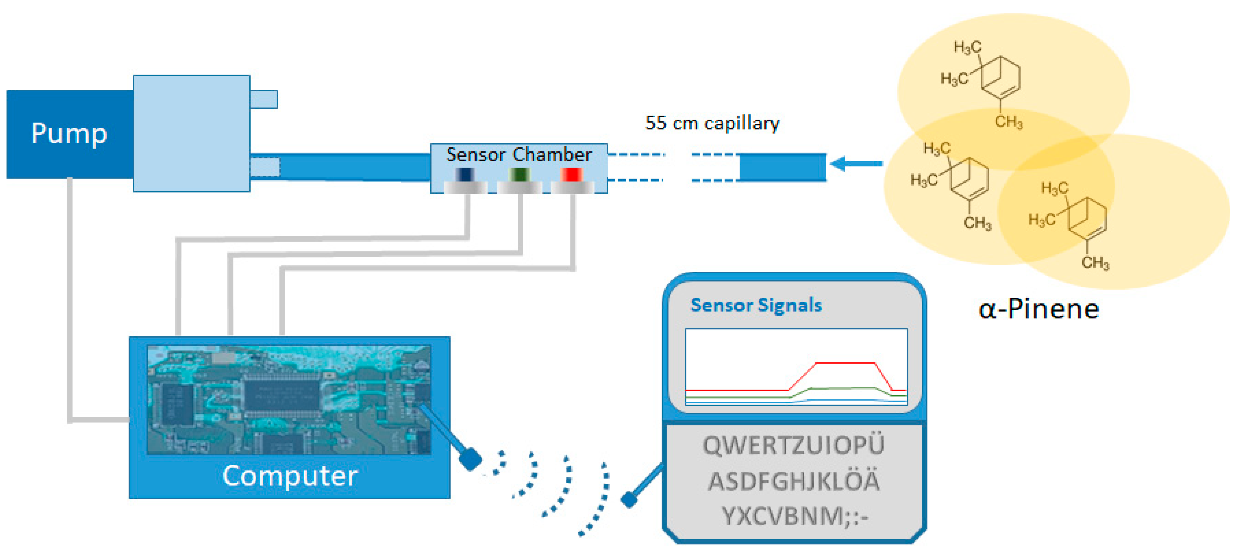
2.1. Sensor Calibration

Synthetic air (100 °C, 1.5 L × min−1, 5.5 purity, 80% N2, 20% O2, Messer Industriegase GmbH, Siegen, Germany) was mixed with a molar 10−2 α-pinene dilution at different flow rates. The α-pinene flow rate was controlled by a syringe pump (LA 30, Landgraf Laborsysteme HLL GmbH, Langenhagen, Germany) at pump rates between 1.5 µL × min−1 to 15 mL × min−1. Due to the constant synthetic air flow, final molar concentrations between 10−8 to 10−4 were mixed. This α-pinene gas flow was led over the surface of three heated metal oxide sensors (GGS1330, metal: SnO2, 450 °C, 5 V, and 26 Ω; GGS2330, metal: SnO3, 400 °C, 4.5 V, and 25 Ω; and GGS5330, metal: WO2, 275 °C, 3 V, and 20.5 Ω; UST Umweltsensortechnik, Geschwenda, Germany) for three minutes, and the conductance was measured (signal processing technology by Cadmium GmbH, Regenstauf, Germany). Between stimuli, the mixing chamber, the heated connection tubes, and the sensor chamber were purged with synthetic air for three minutes.

Data Analysis of Sensor Calibration

Each α-pinene concentration was tested 13 times. The sensor signal decreased under the presence of the stimulus and reached an equilibrium state. This equilibrium state was maintained for three minutes. The mean sensor values of these three minutes were calculated. All mean values per concentration (10−8 to 10−4) and sensor (GGS1330, GGS2330, and GGS5330) were grouped to calculate the mean, standard deviation, median, upper and lower quartiles, minimum and maximum, and the variation coefficient to obtain the indices for signal stability and repeatability of the sensor responses. The mean of the mean values of three-minute stimuli sensor values were used to calculate a linear dose–response correlation for each sensor. All mean values of the three-minute stimuli per sensor were used to calculate a second-grade polynomial function as a dose–response curve for each sensor. This data was also used to calculate the significant differences between adjacent dose–response reactions with the t-test for unpaired samples. The coefficients of determination (R2) were calculated for all dose–response curves as a quality measure for the correlations.

2.2. Sensor Test

A custom-made wind tunnel was adjusted to a linear wind flow of 1 or 2 m × s−1. The sensor, as schematically depicted in Figure 1, was placed at a distance of 1.5 or 3 m on the level of the wind tunnel exit. Either 0.5 or 0.1 mL α-pinene (CAS number: 80-56-8, 98% purity, Merck KgaA, Darmstadt, Germany) were dropped on a filter paper (ROTILABO® Typ 113A, Carl Roth, Stuttgart, Germany), put in a closed petri dish, and placed directly in the wind flow at the exit of the wind tunnel. The sensor was activated, and the petri dish was opened for 3 min and closed for 3 min. This procedure was repeated six times. The first stimulus was not considered for the successive data analysis, as the longer preconcentration time always led to higher sensor signals. After each factor combination (distance, wind flow, and α-pinene concentration), the air in the room was exchanged by a high-performance hood. The factor combinations were repeated at room temperatures of 15 °C, 20 °C, and 25 °C.

Data Analysis of Sensor Test

The combination of the four selected factors resulted in 24 variations. Again, the three-minute equilibrium state of the sensor signals were used to calculate the mean sensor signals. All mean sensor signals were grouped to calculate mean, standard deviation, and correlation coefficient.
The sensor signals of GGS1330 and GGS2330 were related to the signal of GGS5330 in order to normalize the signals and, thus, to increase the comparability of the signals between different trials. This should compensate for the baseline shifts of the sensors and should reduce the effect of the baseline variation between the trials. Significant differences between distance, wind flow, and α-pinene concentration were tested with the t-test for unpaired samples, resulting in 72 pairwise comparisons. The effect of temperature on the sensor signals was analyzed with the Kruskal–Wallis test and the Conover Iman pairwise comparison with Bonferroni adaption, resulting in 16 triple comparisons. The level of significance was p < 0.05.

2.3. Sensor Field Test under Artificial Conditions

A pole that was 4 m high was placed in the botanical garden of the faculty of forest science and forest ecology, University of Göttingen, on 17 March 2020. The sky was clear, and the temperature was 15 °C, with wind speeds below 1 m × s−1 during the trials. A 15 × 20 cm tissue paper with approximately 10 mL of α-pinene was placed at the top of the pole. A drone (Hexacopter, Cadmium GmbH, Regenstauf, Germany) was equipped with the gas sensor system used for the lab experiments. A 55 cm long horizontal glass fiber capillary with a 0.8 mm diameter allowed for air sampling outside the rotor winds (Figure 2). The air was sucked by a pump (1420VP BLDC, Thomas Garden Denver, Fürstenfeldbruck, Germany) through this capillary at 1.5 L × min−1 and was led over the sensor surfaces. The drone was steered manually at approximately 4 m heights over a flat and rectangular area (approximately 40 m × 20 m), with the pole in the center. The minimum distance to the pole was 50 cm from the end of the horizontal capillary. The experiment was repeated one time (N = 1).

Data Analysis of Sensor Field Test under Artificial Conditions

The georeferenced resistance changes of the three sensors were inverted in order to display sensor reactions as upward peaks. The data were displayed as georeferenced dots, with the color indicating the concentration. The georeferenced points with sampled signal intensities were interpolated with the program ArcGIS Geostatistical Analyst (ESRI, Redlands, CA, USA) to a heat map by gradual point overlay and interpolated raster map generation.

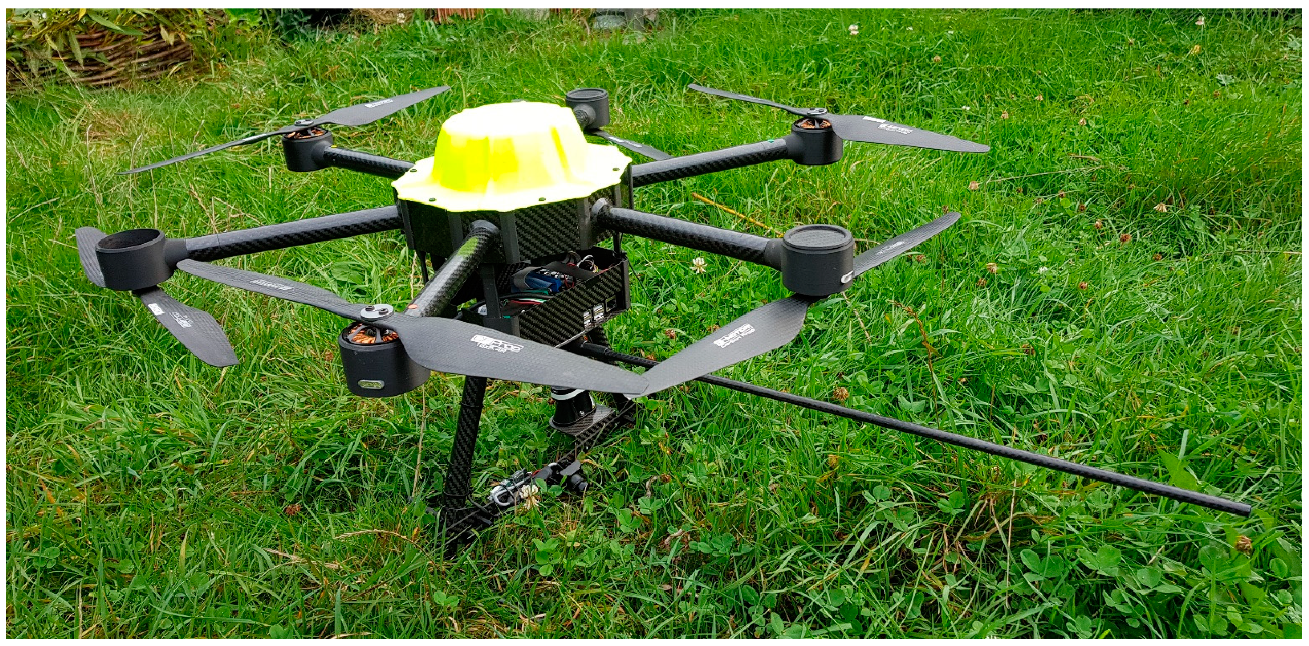
2.4. Sensor Field Test above a Forest Stand

An approximately 40 m × 40 m test stand consisting of 100% spruce trees at different ages between 40 and 80 years at the Windgfällweiher lake, Baden-Württemberg, Germany, was assigned by the forest administration Fürst zu Fürstenberg. The test site was recorded with a multispectral imaging camera (Sequoia Parrot, Pix4D S.A., Prilly, Switzerland) at a height of 80 m with a 90% front and a 80% side overlap in order to create a digital surface model (DSM) with the heights above the ground (drone starting point as reference point) of the forest canopy.
One hundred waypoints were defined over the area, and the assigned height of the waypoints was calculated to be 10 m above the respective heights above the ground, with a lower limit of 20 m. The mikrocopter tool (V2.20, HiSystems GmbH, Moormerland, Germany) was used to transfer the waypoint data to the drone microcontroller.
The weather during the flight mission was slightly cloudy with temperature at 13 °C. The wind was measured with a DJI Mavic 2 Enterprise Zoom (Da-Jiang Innovations Science and Technology Co., Ltd., Nanshan, China) that flew at 27 m heights close to the stand. Wind speed and direction were calculated by a postprocessing IMU (internal measurement unit) data analysis algorithm (AirData, El Dorado Hills, CA, USA). The stand was searched for bark beetle infestation and trees with resin flow caused by physical damage. It was only possible to assess the status of the trees in the lower and middle stem compartments by sight; some trees with many branches in the lower stem compartment could not be completely assessed. All trees in the sampled area were georeferenced using the LogBuch GPS system (SDP Digitale Produkte GmbH, Waiblingen, Germany). The experiment was repeated one time (N = 1).

Data Analysis of Sensor Field Test above a Forest Stand

The DSM was generated by creating digital orthophotos (DOPs) using the software Metashape (V1.6.3, Agisoft, St. Petersburg, Russia). The resulting point cloud was used to calculate the height of each point with the reference of the drone starting position set to 0. In order to highlight damaged trees on the map, individual tree detection (ITD) was performed by identifying local minima in the inverted DSM using the watershed segmentation algorithm (ESRI, Redlands, CA, USA).
The recorded sensor data were displayed with geocoordinates as labels and normalized with the minimum and maximum sensor values for each sensor using R (V.4.0.3, R Core Team). The resulting sensor values were multiplied with each other to obtain a combined sensor response. The sensor values were canopy distance-corrected by assigning weights to the distance of the drone to the canopy in order to compensate for differences between programmed and actual flight paths. The values were normalized again to the mean of the minimum and maximum values to values between −0.75 and 0.26. The georeferenced sensor data were merged with the DSM using ArcGIS Geostatistical Analyst (ESRI, Redlands, CA, USA) to compute an interpolated heat map (universal kriging algorithm assuming autocorrelated errors to trend function): 80% of the sensor data was used to calculate the interpolation, and 20% was used to validate the accuracy of the interpolation.

3. Results

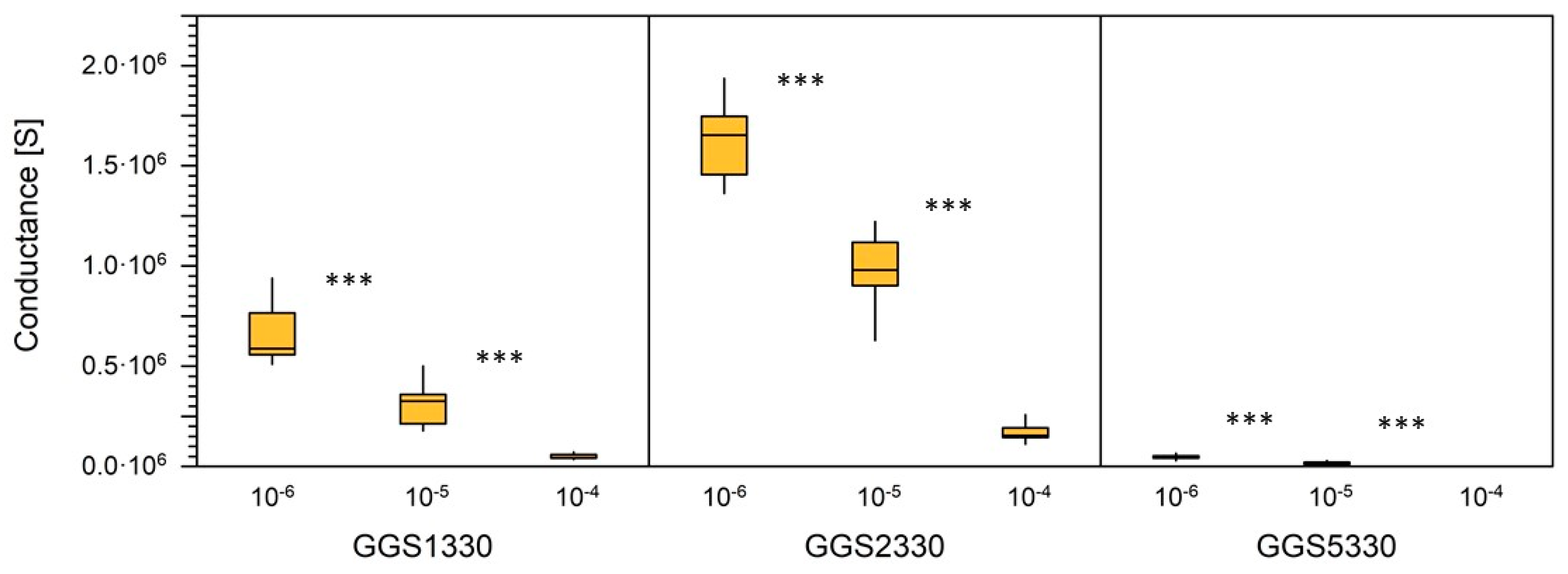
3.1. Sensor Calibration

The results of the sensor calibration are shown in Figure 3. The sensor conductance was increasingly reduced with increasing stimulus concentration, while concentrations below 10−6 did not show a clear and repeatable response and are, therefore, not displayed. At the exposition of the 10−6 concentration, only 7 out of 13 repetitions showed a clear response. The correlation between the stimuli means was very high (Table 2), but the variation in sensor values was high as well (Figure 3 and Table 2). A linear regression showed an acceptable correlation coefficient (Table 2). The GGS2330 showed the highest response to α-pinene.

3.2. Sensor Test under Lab Condition

The sensor test under lab conditions showed low variations in the five stimuli for each parameter combination (Table 3). In general, an increasing temperature decreased the signal relation between GGS1330 and GGS2330 to GGS5330 (Figure 4). Most of these differences were significant or highly significant, with GGS1330 at 0.5 mL, 3 m, and 2 m × s−1 and GGS2330 at 0.5 mL, 3 m, and 2 m × s−1 as the only exceptions. The higher α-pinene amount (0.5 mL) caused a higher signal relation at all temperatures in comparison to 0.1 mL. Out of the 24 compared data sets, 15 data sets (60%) showed significant or highly significant differences.
When using 0.5 mL α-pinene, an increase in the wind flow caused an increased sensor signal relation at 15 °C, while at higher temperatures, the wind flow had a decreasing effect. However, all data sets showed no significant differences between the two wind flows. The distance to the source had an inconsistent effect at 20 °C for six out of eight data sets recorded with 0.5 mL α-pinene. Four data sets showed a significant increase in the values and two showed significant decreases, which showed that there was no repeatable correlation between the two selected distances.
When using 0.1 mL α-pinene, the influence of the wind flow was low. Only two data sets out of 12 showed a significant difference (both GGS1330 and GGS2330 at 20 °C, 0.1 mL, and 1.5 m). At short distance, there was a tendency for higher signal relations (Figure 4), which complemented the tendencies of the 0.5 mL α-pinene amount.

3.3. Sensor Field Test under Artificial Conditions

The sensor field test under artificial conditions showed a response of all three sensors close to the pole with the strong α-pinene source (Figure 5). Sensor GGS1330 showed signals while flying north of the test field, and sensor GGS5330 showed signals scattered over the area. All three sensors responded in the northeast corner of the test field.

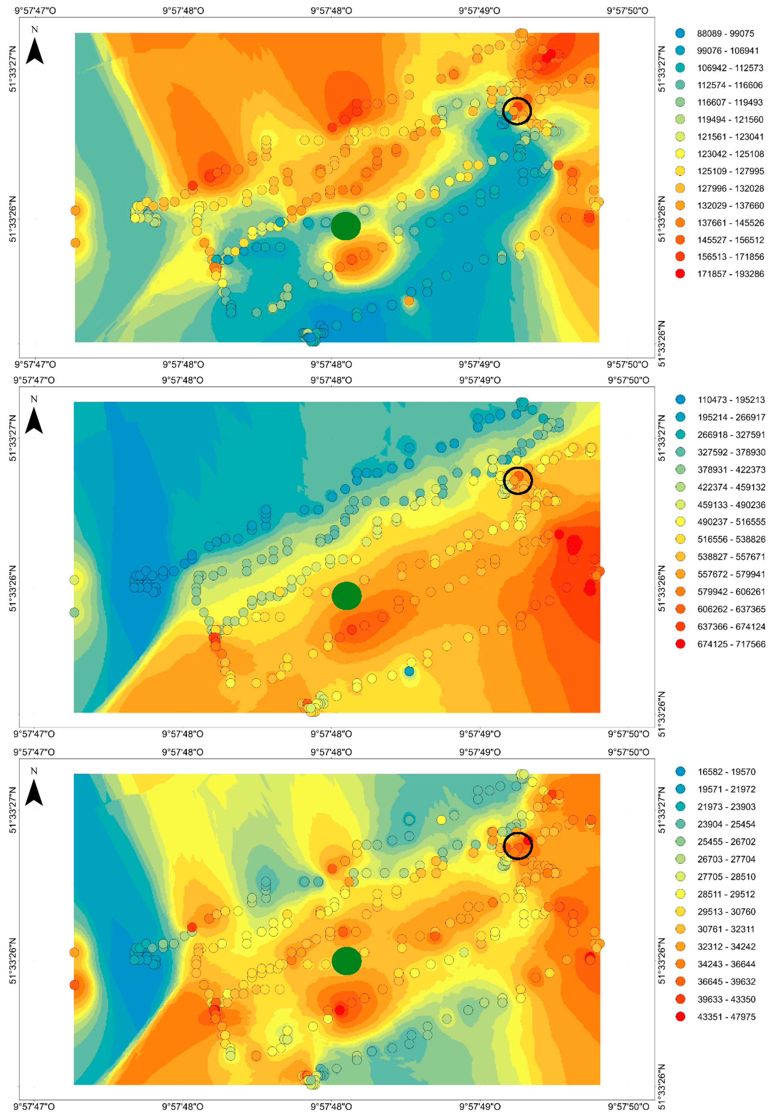
3.4. Sensor Field Test above a Forest Stand

Wind measurement with the drone resulted in an average wind speed of 4.5 m × s−1 from northwest. The heat map was calculated based on an interpolation of all three sensor signals (universal kriging, accuracy R2 = 0.477) and is shown in Figure 6. The calculated tree crown shapes are indicated with black lines. The infested trees and the trees with physical damage, which showed resin flow, are marked with dots.

4. Discussion

The three sensors tested in this study show different response intensities towards α-pinene (Figure 3 and Table 2). The sensor GGS2330 has a SnO3 surface, which allows for the detection of easily thermally oxidizable VOCs. The GGS1330 sensor has a SnO2 surface, which responds to VOCs that are more stable towards thermal oxidization, and the GGS5330 sensor has a WO3 surface, which responds to thermally reducible VOCs. α-Pinene is easily oxidizable at low temperatures [44], which explains the high response of the sensor GGS2330, the lower response of the sensor GGS1330, and the low response of the sensor GGS5330 in Figure 3. GGS2330 had the highest baseline and showed the steepest signal decrease at increasing concentrations, with the highest R2 for the linear correlation of all datapoints (Figure 3 and Table 2). These results correspond to former studies on oak wood emission detection [45] and to a study on the detection of standard chemicals (e.g., 2,4-nonadienal) with SnO2 and WO3 gas sensors [42].
The calibration data were not transformed, so the variation displayed in Figure 1 shows the variation in the raw data and takes into account the differences in the zero-signal values of each sensor at each trial. As the variation coefficients are between 12% to 42%, a reliable field concentration determination can only be achieved by field calibration, e.g., with the method presented by Schultealbert et al. 2017 [46]. However, a relative data analysis as presented in Figure 4 can be sufficient to identify infested trees, which can be located by the relative signal increase. Such an approach was demonstrated by Sauerwald in Paczkowski et al. [30] for thermally treated wood flakes. The highly significant differences between the factor 10 dilutions in Figure 3 suggest that the differentiation capacities of all three sensors are below a factor 10 difference in the range between 10−4 and 10−6. According to Kohl et al., a differentiation of a factor 2 difference is possible at a 10−6 concentration of 2,4-nonadienal detected with a ZnO/SnO2 sensor [42]. A study by Schüler et al. suggests that, under lab conditions, a much higher sensitivity in the sub ppb range accompanied by a good selectivity can be possible [47].
As described in Section 2.1 of this article, the sensors were run with constant heater resistances both in the lab and field experiments. These resistances can be changed and adapted to the detection of monoterpenes, including α-pinene, in order to further improve both the selectivity and the sensitivity of the sensor system [48]. An example of the impact of the heater resistance on the sensor signal by induced sensor surface temperature alternation is given by Sauerwald in Paczkowski et al. 2013 [30]. Temperature cycles over the sensor surface increased the signal selectivity, as selected temperatures showed a compound-specific response pattern. This concept can be used to improve detection by increasing the selectivity towards monoterpenes, including α-pinene, in complex gas mixtures. However, such gas mixtures would be rare above conifer forests, as, e.g., Giunta et al. [27] and Page et al. [25,26] both only found terpenes in the VOC pattern of healthy and infested conifer trees.
It is not possible to detect bark beetle pheromones with semiconductor gas sensors. As shown in Erbilgin et al. [38] the pheromone concentrations are far below the expected α-pinene levels at ratios between 50:1 to 5000:1. Under such circumstances, the α-pinene oxidation on the sensor surface will strongly superimpose the pheromone-induced conductance change, which will disable pheromone detection. This is one of many examples that show the lack of selectivity of semiconductor gas sensors [42]. Bark beetles derive a sensitive and selective biological VOC detection system based on odor-specific odor-binding proteins [31,34,39,40,42]. This allows the beetles to communicate on the basis of low pheromone concentrations in complex odor mixtures [38]. At present, it is not possible to use OBPs on sensor surfaces for reliable odor detection under field conditions [49].
Six out of 12 data sets showed significant differences between the two distances in the lab experiment (Table 2 and Figure 2). In three cases, the correlations were positive, and in three cases, the correlations were negative. Therefore, these significances are considered nonexplanatory. Apparently, the difference in the distances between 1.5 m and 3 m is neglectable from a practical point of view. Probably, complex odor dispersion is responsible for the contradictive results, as plumes of odor show a high spatial concentration distribution that is weakly correlated to the distance from the source [50,51,52,53]. A significant dilution of α-pinene will only occur at larger distances, which corresponds to studies on VOC dispersion in nature [50,54]. This indicates that temperature and source concentration determine the emission rate at short ranges between 1.5 m and 3 m and low wind speeds of 1 m × s−1 and 2 m × s−1 (Figure 4).
Relating this information to field conditions, the limit of detecting the first generation of bark beetles in spring will be the environmental temperature at this time of the year. As the flight time of the bark beetles can start at low degrees, the first attack of the bark beetle might not be detectable at all. In this case, secondary plant stress emissions can serve as cues for infestation after an early initial infestation. Also, bark beetles attracted by the pheromones of the first successful bark beetles can cause additional resin flow after an early initial infestation.
VOC vapor pressure is positively correlated with temperature (Clausius Clapeyron relation), while bark beetle breeding cycle time is negatively correlated with temperature [8]. Therefore, a warm and dry spring season will facilitate both beetle development and the detection probability of monoterpenes, e.g., α-pinene. Increasing temperatures in the course of the season will further improve the detectability of bark beetle infestation at an early stage by means of monoterpene emissions [2,8]. This concept can be compromised by stands under initial drought stress, which will emit increased amounts of monoterpenes such as α-pinene even if they are not affected by bark beetle infestation [22,24] (Table 1). This emission increase in the initial drought stage is caused by a higher temperature and a successive increasing vapor pressure of α-pinene. In such cases, the background level of monoterpenes could be too high to differentiate between infested and not infested trees.
Table 1 shows that the overall emission differences between infested and healthy trees can be high. The data in the table also show few exceptions, which indicates a variable emission response to infestation. Further research has to address and clarify this issue, and the proposed drone system can help establish a large data basis, either with sensor data or, e.g., with a sorbent tube sampling method and a successive laboratory analysis.
Stands weakened by drought stress will have a higher probability of intense and uncontrollable bark beetle infestations, so the proposed drone-based sensor detection concept with single tree identification is not practical (Table 1). After a longer drought period, the trees will emit less terpenes [22] (Table 1) and start to increase the terpene levels inside the needle and wood tissue due to stomata closure [24]. Stands under strong and continuous drought stress lose their ability to resinate, as the trees are less physiological active [25,26,27] and lose their ability to produce monoterpene cyclase [29]. Such stands are usually severely attacked by bark beetles [28], and the proposed detection concept is not applicable under these extreme circumstances. The drone-based sensor concept is applicable for healthy trees under initial bark beetle attack [28].
Table 1 shows the literature values on monoterpene and α-pinene emission from conifer trees. In most cases of bark beetle infestation, the emission ratio increases between 1.4–5.1, which shows a higher emission rate after the infestation. However, there are some inconsistencies in the literature. Page et al. reported an increase in the emission rate in the yellow stage after infestation [26], while in an earlier study, applying the same method resulted in increasing emissions in the green infested stage [25] (Table 1). Ormeno et al. sampled drought stress emissions of Pinus halepensis seedlings, and the result was a fluctuation of the emission ratio throughout the experiment (Table 1). The absolute values given by the authors should not be compared between studies using different methods. For instance, Ormeno et al. [24] and Blanch et al. [22] used three- and two-year-old seedlings for their drought experiments, respectively, while Page et al. used the lower branches of adult trees [25,26]. Amin et al. [28] sampled in the crown and compared the α-pinene emissions with the trunk emissions. The authors of this study found that the emission difference between infested and not infested trees are higher in the trunk, as the bark beetles attack this tree compartment directly. The α-pinene emitted at the trunk diffuses to the crown, where it is present at lower concentrations. A general stress response can add to these emissions by stomata gas exchange of monoterpenes [20,21,29]. The studies summarized in Table 1 indicate that the emission dynamic of infested trees is complex. The comparison between infestation-induced and drought-induced terpene emission shows that the assumptions on the limitations of the drone-based early bark beetle infestation presented above are reasonable. Intense drought can disable the possibility to detect bark beetle infestation at an early stage.
The sensor calibration data shown in Figure 3 and Table 2 can be displayed as an emission rate. In a comparative approach, the resulting values match the proposed emission intensities in Table 1 (sensor response at 10−6 equals 90 ng × h−1 or 1 ng × L−1). This does not take into consideration that the data in Table 1 are related to only one gram of dry or fresh biomass. Eighty-year-old spruce trees have a crown mass of approximately 40 kg [55]. Although these calculations are based on studies with different methodological approaches, there is a resemblance between the expected emissions from infested trees and sensor sensitivity. Additionally, there is a high order of magnitude between the sampled emissions from 1 g of biomass in the experiments listed in Table 1 and the expected amount of biomass in the field. This supports the feasibility of the drone-based sensor approach for early detection of bark beetle infestation.
Although the drone was able to locate the strong α-pinene source in Figure 5 (green dot), it also located another source (black circle). This source was a prunus domestica tree that caused a signal increase in the inverted signal. Trees emit isoprene and other volatile compounds during leave and bud development [56,57]. It is probable that the increasing physiological activity of the broad leave tree in march caused the weak signal in Figure 3 (black circle). These results confirm the measuring concept. However, false identifications are possible depending on the emission of monoterpenes or other VOCs. In cases where unspecific emissions of monoterpenes from plants are needed, e.g., for forest/atmosphere interactions [16,17,18,20], the sensor can provide valuable information for small-scale analysis or upscaling model approaches. It also allows us to investigate diurnal emission differences [18] or climate dependent emission dynamics [20,21,29]. In Figure 5, the interpolation of the sensor data led to artifact signals at larger distances to the sensor signal points, which did not correspond to high VOC concentrations.
Other sources of false positive sensor signals can be logging sites or trees broken by storm or ice, which emit very high concentrations of α-pinene. This suggests that the assessment of VOC emission is not enough to differentiate between false positive and positive signals. Optical assessments by drones, planes, or even satellite can add valuable information to identify the emission source. However, false-positive detections cannot be completely excluded.
The field trial was performed under unfavorable conditions, as the temperature was low and the wind was relatively strong (Ø: 4.5 m × s−1 or 8.7 knots), blowing northwest. Due to GPS inaccuracy the drone deviated from the programmed flight path and, therefore, maneuvered between 5 m and 15 m above the calculated DSM. This is both too high and too variable for consistent VOC detection performance. Therefore, the results in the heat map (Figure 6) have to be considered preliminary. It has to be mentioned that northwest of all bark beetle-infested trees there is a signal increase at a constant distance to the potential source, which could be caused by monoterpenes, especially α-pinene, that were emitted and distributed by the wind to the northwest. Due to the restrictions described above, there were many signal increases over the area. Therefore, consistency of the signal increases northwest of the sources does not confirm the measuring concept.
Bark beetle detection can only be performed during spring and summer, when the beetle is active and the temperatures are elevated. Therefore, no distinct correlation between the positions of the infested trees and the sensor signals are visible in Figure 6. It is possible that other sources, e.g., damaged twigs that were not visible from the ground or in the aerial survey, had an impact on the VOC distribution. The field trials have to be repeated at warmer temperatures, e.g., in springtime 2021, and under less wind influence. An improved GPS system, e.g., an RTK (real-time kinematic) GPS, has to ensure guidance of the drone along the precalculated flight path to maintain a constant distance above the canopy surface. Improved drone distance sensors that can detect small geometric structures, e.g., small branches and twigs, will allow the drone to fly closer to the canopies. This will improve the signal noise ratio of the monoterpene detection.
An economic feasibility study of the new bark beetle detection system (unpublished) showed that the drone sensor approach will be financially competitive against conventional early bark beetle detection by sight in steep areas, in areas with dense understory, and for large areas. The average costs per ha were estimated to be below 60 USD. Multiple flights throughout the vegetation period will be necessary in order to effectively prevent bark beetle gradation.

5. Conclusions

The drone-based semiconductor metal oxide sensor array is a promising new technology that allows for sampling of volatile emissions in the air. α-Pinene was detectable as an artificial source by a drone-based gas sensor, but the proof of principle above forest stands with trees in an early infestation stage still has to be performed. Technical barriers are the drone technology (close canopy flight by high-precision GPS and distance sensors) and the sensor selectivity. Further research will also address the VOC distribution dynamics in forest stands to understand the relation between detected VOCs above the crown and the position of infested trees under wind influence. The drone-based sensor can play an important role in understanding forest borne monoterpene emissions from an atmospheric research perspective. The approach can yield improved data for precision modeling, e.g., of drought stress-induced atmospheric emissions of forest stands.

Author Contributions

Conceptualization, S.P. (Sebastian Paczkowski) and P.D.; methodology, S.P. (Sebastian Paczkowski), P.D., M.P., T.H., H.I., and D.J.; software, P.D., H.I., and M.P.; validation, S.P. (Sebastian Paczkowski), T.H., and D.J.; formal analysis, S.P. (Sebastian Paczkowski), H.I., P.D., M.P., and T.H.; investigation, S.P. (Sebastian Paczkowski), P.D., H.I., and M.P.; resources, D.J. and S.P. (Sebastian Paczkowski); data curation, H.I. and M.P.; writing—original draft preparation, S.P. (Sebastian Paczkowski), P.D., and D.J.; writing—review and ed-iting, S.P. (Sebastian Paczkowski) and P.D.; visualization, S.P. (Sebastian Paczkowski), M.P., P.D., and H.I.; supervision, D.J. and S.P. (Sebastian Paczkowski); project ad-ministration, S.P. (Sebastian Paczkowski), P.D., D.J., and S.P. (Stefan Pelz); funding acquisition, S.P. (Sebastian Paczkowski), D.J., and S.P. (Stefan Pelz). All authors have read and agreed to the published version of the manuscript.

Funding

This research was funded by the FNR—Fachagentur für Nachwachsende Rohstoffe, Germany, under the grant number 22011018.

Institutional Review Board Statement

Not applicable.

Informed Consent Statement

Not applicable.

Data Availability Statement

The data presented in this study are available on request from the corresponding author.

Acknowledgments

The authors want to thank the forest owners Graf Ferdinand v. Drechsel, Christian Vogt, and Christian Fürst zu Fürstenberg and the forest manager Dietrich Nübling for their cooperation considering the field tests and the team of Cadmium GmbH for their technical support.

Conflicts of Interest

The authors declare that they have no competing financial interests or personal relationships that could have influenced the work reported in this paper.

References

  1. De Grandpré, L.; Pureswaran, D.; Bouchard, M.; Kneeshaw, D. Climate-induced range shifts in boreal forest pests: Ecological, economic, and social consequences. Can. J. For. Res. 2018, 48, v–vi. [Google Scholar] [CrossRef] [Green Version]
  2. Rouault, G.; Candau, J.-N.; Lieutier, F.; Nageleisen, L.-M.; Martin, J.-C.; Warzée, N. Effects of drought and heat on forest insect populations in relation to the 2003 drought in Western Europe. Ann. For. Sci. 2006, 63, 613–624. [Google Scholar] [CrossRef]
  3. Corbett, L.J.; Withey, P.; Lantz, V.A.; Ochuodho, T.O. The economic impact of the mountain pine beetle infestation in British Columbia: Provincial estimates from a CGE analysis. Forestry 2016, 89, 100–105. [Google Scholar] [CrossRef] [Green Version]
  4. Dale, V.; Joyce, A.L.; McNulty, S.; Neilson, R.P.; Ayres, M.P.; Flannigan, M.D.; Hanson, P.J.; Irland, L.C.; Lugo, A.E.; Peterson, C.J.; et al. Climate change and forest disturbances. BioScience 2001, 51, 723–734. [Google Scholar] [CrossRef] [Green Version]
  5. Bundesministerium für Ernährung und Landwirtschaft. Waldschäden: Bundesministerium Veröffentlicht Aktuelle Zahlen. Available online: https://www.bmel.de/SharedDocs/Pressemitteilungen/DE/2020/040-waldschaeden.html;jsessionid=E322EBC9C439CDFD426657E41A3E9DC5.internet2851 (accessed on 1 July 2020).
  6. Bundesministerium für Ernährung und Landwirtschaft. Bundeswaldinventur. Available online: https://bwi.info/inhalt1.3.aspx?Text=3.05%20Altersklasse&prRolle=public&prInv=BWI2012&prKapitel=3.05 (accessed on 10 October 2020).
  7. McCollum, D.W.; Lundquist, J.E. Bark Beetle Infestation of Western US Forests: A Context for Assessing and Evaluating Impacts. J. Forest. 2019, 117, 171–177. [Google Scholar] [CrossRef]
  8. Wermelinger, B.; Seifert, M. Temperature-dependent reproduction of the spruce bark beetle Ips typographus, and analysis of the potential population growth. Ecol. Entomol. 1999, 24, 103–110. [Google Scholar] [CrossRef]
  9. Immitzer, M.; Einzmann, K.; Pinnel, N.; Seitz, R.; Atzberger, C. Vitaliltätserfassung von Fichten mittels Fernerkundung. AFZ Wald 2018, 17, 20–23. [Google Scholar]
  10. Anderbrant, O. Reemergence and Second Brood in the Bark Beetle Ips typographus. Holartic Ecol. 1989, 12, 494–500. [Google Scholar] [CrossRef]
  11. Thatcher, C.R. The Southern Pine Beetle; United State Department of Agriculture: Washington, DC, USA, 1981. [Google Scholar]
  12. Schwerdtfeger, F. Waldkrankheiten; Paul Parey: Hamburg/Berlin, Germany, 1970. [Google Scholar]
  13. Lausch, A.; Heurich, M.; Gordalla, D.; Dobner, H.-J.; Gwillym-Margianto, S.; Salbach, C. Forecasting potential bark beetle outbreaks based on spruce forest vitality using hyperspectral remote-sensing techniques at different scales. Forest. Ecol. Manag. 2013, 308, 76–89. [Google Scholar] [CrossRef]
  14. Fassnacht, F.E.; Latifi, H.; Ghosh, A.; Joshi, P.K.; Koch, B. Assessing the potential of hyperspectral imagery to map bark beetle-induced tree mortality. Remote Sens. Environ. 2014, 140, 533–548. [Google Scholar] [CrossRef]
  15. Hais, M.; Wild, J.; Berec, L.; Brůna, J.; Kennedy, R.; Braaten, J.; Brož, Z. Landsat Imagery Spectral Trajectories—Important Variables for Spatially Predicting the Risks of Bark Beetle Disturbance. Remote Sens. Environ. 2016, 8, 687. [Google Scholar] [CrossRef] [Green Version]
  16. Guenther, A.; Hewitt, C.N.; Erickson, D.; Fall, R.; Geron, C.; Graedel, T.; Harley, P.; Klinger, L.; Lerdau, M.; Mckay, W.A.; et al. A global model of natural volatile organic compound emissions. J. Geophys. Res. 1995, 100, 8873. [Google Scholar] [CrossRef]
  17. Isidorov, V.A.; Zenkevich, I.G.; Ioffe, B.V. Volatile organic compounds in the atmosphere of forests. Atmos. Environ. 1985, 19, 1–8. [Google Scholar] [CrossRef]
  18. Enders, G.; Dlugi, R.; Steinbrecher, R.; Clement, B.; Daiber, R.; Euk, J.; Gäb, S.; Haziza, M.; Helas, G.; Herrmann, U.; et al. Biosphere/Atmosphere interactions: Integrated research in a European coniferous forest ecosystem. Atmos. Environ. 1992, 26, 171–189. [Google Scholar] [CrossRef]
  19. Berg, A.R.; Heald, C.L.; Huff Hartz, K.E.; Hallar, A.G.; Meddens, A.J.H.; Hicke, J.A.; Lamarque, J.-F.; Tilmes, S. The impact of bark beetle infestations on monoterpene emissions and secondary organic aerosol formation in western North America. Atmos. Chem. Phys. 2013, 13, 3149–3161. [Google Scholar] [CrossRef] [Green Version]
  20. Lerdau, M.; Dilts, S.B.; Westberg, H.; Lamb, B.K.; Allwine, E.J. Monoterpene emission from ponderosa pine. J. Geophys. Res. 1994, 99, 16609. [Google Scholar] [CrossRef]
  21. Yokouchi, Y.; Ambe, Y. Factors Affecting the Emission of Monoterpenes from Red Pine (Pinus densiflora). Plant. Physiol. 1984, 75, 1009–1012. [Google Scholar] [CrossRef] [Green Version]
  22. Blanch, J.-S.; Peñuelas, J.; Llusià, J. Sensitivity of terpene emissions to drought and fertilization in terpene-storing Pinus halepensis and non-storing Quercus ilex. Physiol. Plant. 2007, 131, 211–225. [Google Scholar] [CrossRef]
  23. Holopainen, J.K. Multiple functions of inducible plant volatiles. Trends Plant. Sci. 2004, 9, 529–533. [Google Scholar] [CrossRef] [PubMed]
  24. Ormeño, E.; Mévy, J.P.; Vila, B.; Bousquet-Mélou, A.; Greff, S.; Bonin, G.; Fernandez, C. Water deficit stress induces different monoterpene and sesquiterpene emission changes in Mediterranean species. Relationship between terpene emissions and plant water potential. Chemosphere 2007, 67, 276–284. [Google Scholar] [CrossRef] [Green Version]
  25. Page, W.G.; Jenkins, M.J.; Runyon, J.B. Mountain pine beetle attack alters the chemistry and flammability of lodgepole pine foliage. Can. J. For. Res. 2012, 42, 1631–1647. [Google Scholar] [CrossRef] [Green Version]
  26. Page, W.G.; Jenkins, M.J.; Runyon, J.B. Spruce Beetle-Induced Changes to Engelmann Spruce Foliage Flammability. For. Sci. 2014, 60, 691–702. [Google Scholar] [CrossRef] [Green Version]
  27. Giunta, A.D.; Runyon, J.B.; Jenkins, M.J.; Teich, M. Volatile and Within-Needle Terpene Changes to Douglas-fir Trees Associated With Douglas-fir Beetle (Coleoptera: Curculionidae) Attack. Environ. Entomol. 2016, 45, 920–929. [Google Scholar] [CrossRef]
  28. Amin, H.; Atkins, P.T.; Russo, R.S.; Brown, A.W.; Sive, B.; Hallar, A.G.; Huff Hartz, K.E. Effect of bark beetle infestation on secondary organic aerosol precursor emissions. Environ. Sci. Technol. 2012, 46, 5696–5703. [Google Scholar] [CrossRef] [PubMed]
  29. Lewinsohn, E.; Gijzen, M.; Croteau, R. Defense Mechanisms of Conifers Differences in Constitutive and Wound-Induced Monoterpene Biosynthesis Among Species. Plant. Physiol. 1991, 96, 44–49. [Google Scholar] [CrossRef] [PubMed] [Green Version]
  30. Paczkowski, S.; Paczkowska, M.; Dippel, S.; Schulze, N.; Schütz, S.; Sauerwald, T.; Weiß, A.; Bauer, M.; Gottschald, J.; Kohl, C.-D. The olfaction of a fire beetle leads to new concepts for early fire warning systems. Sens. Actuat. B Chem. 2013, 183, 273–282. [Google Scholar] [CrossRef]
  31. Blomquist, G.J.; Figueroa-Teran, R.; Aw, M.; Song, M.; Gorzalski, A.; Abbott, N.L.; Chang, E.; Tittiger, C. Pheromone production in bark beetles. Insect Biochem. Mol. Biol. 2010, 40, 699–712. [Google Scholar] [CrossRef]
  32. Hedgren, P.O. The bark beetle Pityogenes chalcographus (L.) (Scolytidae) in living trees: Reproductive success, tree mortality and interaction with Ips typographus. J. Appl. Entomol. 2004, 128, 161–166. [Google Scholar] [CrossRef]
  33. Byers, J.A.; Wood, D.L. Interspecific effects of pheromones on the attraction of the bark beetles, Dendroctonus brevicomis and Ips paraconfusus in the laboratory. J. Chem. Ecol. 1981, 7, 9–18. [Google Scholar] [CrossRef] [PubMed]
  34. Tittiger, C.; Blomquist, G.J. Pheromone biosynthesis in bark beetles. Curr. Opin. Insect Sci. 2017, 24, 68–74. [Google Scholar] [CrossRef]
  35. Byers, J.A. Chemical ecology of bark beetles. Experientia 1989, 45, 271–283. [Google Scholar] [CrossRef]
  36. Gitau, C.W.; Bashford, R.; Carnegie, A.J.; Gurr, G.M. A review of semiochemicals associated with bark beetle (Coleoptera: Curculionidae: Scolytinae) pests of coniferous trees: A focus on beetle interactions with other pests and their associates. For. Ecol. Manag. 2013, 297, 1–14. [Google Scholar] [CrossRef]
  37. Progar, R.A.; Gillette, N.; Fettig, C.J.; Hrinkevich, K. Applied Chemical Ecology of the Mountain Pine Beetle. For. Sci. 2014, 60, 414–433. [Google Scholar] [CrossRef]
  38. Erbilgin, N.; Powell, J.S.; Raffa, K.F. Effect of varying monoterpene concentrations on the response of Ips pini (Coleoptera: Scolytidae) to its aggregation pheromone: Implications for pest management and ecology of bark beetles. Agric. For. Ent. 2003, 5, 269–274. [Google Scholar] [CrossRef] [Green Version]
  39. Andersson, M.N.; Grosse-Wilde, E.; Keeling, C.I.; Bengtsson, J.M.; Yuen, M.M.S.; Li, M.; Hillbur, Y.; Bohlmann, J.; Hansson, B.S.; Schlyter, F. Antennal transcriptome analysis of the chemosensory gene families in the tree killing bark beetles, Ips typographus and Dendroctonus ponderosae (Coleoptera: Curculionidae: Scolytinae). BMC Genom. 2013, 14, 198. [Google Scholar] [CrossRef] [Green Version]
  40. Yuvaraj, J.K.; Roberts, R.E.; Sonntag, Y.; Hou, X.-Q.; Grosse-Wilde, E.; Machara, A.; Zhang, D.-D.; Hansson, B.S.; Johanson, U.; Löfstedt, C.; et al. Putative ligand binding sites of two functionally characterized bark beetle odorant receptors. BMC Biol. 2021, 19, 16. [Google Scholar] [CrossRef]
  41. Pelosi, P. Odorant-binding proteins. Crit. Rev. Biochem. Mol. Biol. 1994, 29, 199–228. [Google Scholar] [CrossRef]
  42. Kohl, D.; Heinert, L.; Bock, J.; Hofmann, T.; Schieberle, P. Systematic studies on responses of metal-oxide sensor surfaces to straight chain alkanes, alcohols, aldehydes, ketones, acids and esters using the SOMMSA approach. Sens. Actuat. B Chem. 2000, 70, 43–50. [Google Scholar] [CrossRef]
  43. Krüll, W.; Tobera, R.; Willms, I.; Essen, H.; von Wahl, N. Early Forest Fire Detection and Verification using Optical Smoke, Gas and Microwave Sensors. Procedia Eng. 2012, 45, 584–594. [Google Scholar] [CrossRef]
  44. Neuenschwander, U.; Guignard, F.; Hermans, I. Mechanism of the Aerobic Oxidation of α-Pinene. ChemSusChem 2010, 3, 75–84. [Google Scholar] [CrossRef]
  45. Paczkowski, S.; Pelz, S.; Jaeger, D. Semi-conductor metal oxide gas sensors for online monitoring of oak wood VOC emissions during drying. Dry. Technol. 2019, 37, 1081–1086. [Google Scholar] [CrossRef]
  46. Schultealbert, C.; Baur, T.; Schütze, A.; Böttcher, S.; Sauerwald, T. A novel approach towards calibrated measurement of trace gases using metal oxide semiconductor sensors. Sens. Actuat. B Chem. 2017, 239, 390–396. [Google Scholar] [CrossRef]
  47. Schüler, M.; Helwig, N.; Ventura, G.; Schütze, A.; Sauerwald, T. IEEE Sensors, Proceedings of the 12th IEEE Sensors Conference, Baltimore, Maryland, USA, 3–6 November 2013; IEEE: Piscataway, NJ, USA, 2013; ISBN 9781467346405. [Google Scholar]
  48. Leidinger, M.; Sauerwald, T.; Conrad, T.; Reimringer, W.; Ventura, G.; Schütze, A. Selective Detection of Hazardous Indoor VOCs Using Metal Oxide Gas Sensors. Proc. Engin. 2014, 87, 1449–1452. [Google Scholar] [CrossRef] [Green Version]
  49. Bohbot, J.D.; Vernick, S. The Emergence of Insect Odorant Receptor-Based Biosensors. Biosensors 2020, 10, 26. [Google Scholar] [CrossRef] [PubMed] [Green Version]
  50. Meng, Q.-H.; Yang, W.-X.; Wang, Y.; Li, F.; Zeng, M. Adapting an ant colony metaphor for multi-robot chemical plume tracing. Sensors 2012, 12, 4737–4763. [Google Scholar] [CrossRef] [PubMed]
  51. de Croon, G.; O’Connor, L.M.; Nicol, C.; Izzo, D. Evolutionary robotics approach to odor source localization. Neurocomputing 2013, 121, 481–497. [Google Scholar] [CrossRef]
  52. Monroy, J.; Hernandez-Bennets, V.; Fan, H.; Lilienthal, A.; Gonzalez-Jimenez, J. GADEN: A 3D Gas Dispersion Simulator for Mobile Robot Olfaction in Realistic Environments. Sensors 2017, 17, 1479. [Google Scholar] [CrossRef] [Green Version]
  53. Ishida, H.; Wada, Y.; Matsukura, H. Chemical Sensing in Robotic Applications: A Review. IEEE Sens. J. 2012, 12, 3163–3173. [Google Scholar] [CrossRef]
  54. Balkovsky, E.; Shraiman, B.I. Olfactory search at high Reynolds number. Proc. Natl. Acad. Sci. USA 2002, 99, 12589–12593. [Google Scholar] [CrossRef] [PubMed] [Green Version]
  55. Turski, M.; Beker, C.; Kazmierczak, K.; Najgrakowski, T. Allometric equations for estimating the mass and volume of fresh assimilational apparatus of standing scots pine (Pinus sylvestris L.) trees. For. Ecol. Manag. 2008, 255, 2678–2687. [Google Scholar] [CrossRef]
  56. Li, Y.; Ma, H.; Wan, Y.; Li, T.; Liu, X.; Sun, Z.; Li, Z. Volatile Organic Compounds Emissions from Luculia pinceana Flower and Its Changes at Different Stages of Flower Development. Molecules 2016, 21, 531. [Google Scholar] [CrossRef] [PubMed] [Green Version]
  57. Kuhn, U.; Rottenberger, S.; Biesenthal, T.; Wolf, A.; Schebeske, G.; Ciccioli, P.; Kesselmeier, J. Strong correlation between isoprene emission and gross photosynthetic capacity during leaf phenology of the tropical tree species Hymenaea courbaril with fundamental changes in volatile organic compounds emission composition during early leaf development. Plant. Cell Environ. 2004, 27, 1469–1485. [Google Scholar] [CrossRef]
Figure 1. Schematic sensor setup that was used in the laboratory experiment (see Section 2.2) and that was attached to the drone for the field tests (see Section 2.3 and Section 2.4).
Forests 12 00228 g001
Figure 2. Picture of the PROTECTFOREST drone with the sensor system and capillary.
Forests 12 00228 g002
Figure 3. Sensor response (median, upper and lower quartiles, minimum, and maximum) to three concentrations of α-pinene (10−6, 10−5, and 10−4) for each sensor (GGS1330, GGS2330, and GGS5330), with N = 13: the conductance was reduced with increasing stimulus concentration. Concentrations below 10−6 are not shown as they did not elicit a sensor response. Significant differences between responses to adjacent concentrations were calculated with the t-test for unpaired samples and are indicated by stars (*** p < 0.001).
Forests 12 00228 g003
Figure 4. Sensor response of GGS1330 and GGS2330 in relation to GGS5330 (dimensionless) at different temperatures (°C) for the selected factor combinations of α-pinene amount (mL), distance to α-pinene source (m), and wind speed (m × s−1). Lines between the points do not indicate interpolation but improve readability. N was 5 for all combinations.
Forests 12 00228 g004
Figure 5. The heat maps generated from the inverted and interpolated sensor signals in conductance (S) (from top: GGS1330, GGS2330, and GGS5330, with N = 1): the sensors were attached to a drone that flew over a plane field with an α-pinene source held by a pole at 4 m heights (green dot). A prunus domestica tree is marked with a circle. Red indicates a high sensor response, and blue indicates a low sensor response.
Forests 12 00228 g005
Figure 6. The sensor signal heat map (inverted, normalized, all three sensor values multiplied, and height above crown corrected and interpolated by universal kriging with R2 = 0.477) with the calculated tree crown geometries (inverted DSM with the watershed algorithm) and manual assignment of the infested trees and trees that show resin flow from physical damage (visual stand assessment at the site). N = 1.
Forests 12 00228 g006
Table 1. Emission comparison between infested and not infested tree species (above) and emission comparison between tree species with and without drought stress (below) in the literature. a Emission ratio = emission (infested or drought stress)/emission (not infested or no drought stress). b The green infested stage always showed lower emission in comparison to the not infested stage.
Tree Species
(Specification)
Compound
(Unit)
Emission
(Not Infested)
Emission
(Infested)
Infestation StageEmission Ratio aSource
Pinus contorta
(canopy)
α-pinene
(ng × L−1)
1.1 ± 0.56 1.5 ± 0.6unknown1.4[28]
2.6 ± 0.92.7 ± 1.11.0
Pseudotsuga menziesii (lower branches)α-pinene
(ng × h−1 × gFM−1)
322 ± 166 813 ± 482Green2.5[27]
Pseudotsuga menziesii (lower branches)Total terpenes
(ng × h−1 × gFM−1)
870 ± 417 4472 ± 2759Green5.1[27]
1515 ± 7371472 ± 8341.0
1695 ± 7975881 ± 36853.4
571 ± 2262480 ± 10944.3
284 ± 59462 ± 1891.6
557 ± 251229 ± 680.4
842 ± 268724 ± 2430.9
948 ± 6842124 ± 17822.2
Pseudotsuga menziesii (lower branches)α-pinene
(ng × h−1 × gFM−1)
77190Yellow b2.5[26]
1001901.9
601342.2
701842.6
Tree SpeciesCompoundEmission
(No Draught)
Emission (Draught)Draught IntensityEmission Ratio aSource
Pinus
halepensis
(seedlings)
α-pinene
(µg × h−1 × gDM−1)
23.9 ± 5.8 17.9 ± 1.32 weeks0.7[22]
5.6 ± 0.716.4 ± 5.34 weeks2.9[22]
8.8 ± 3.24.0 ± 1.36 weeks0.5[22]
30.7 ± 4.520.6 ± 4.88 weeks0.7[22]
10.9 ± 4.521.2 ± 5.810 weeks1.9[22]
34.2 ± 7.521.4 ± 4.812 weeks0.6[22]
Pinus
halepensis
(seedlings)
α-pinene
(%total VOC)
30.8 ± 10.6 60.0 ±14.31 week1.9[24]
Table 2. Descriptive statistics (mean, standard deviation, and variation coefficient) and dose–response curve regression analysis with coefficients of determination (R2) of the sensor responses (mean value over a three-minute stimulus) to the selected α-pinene dilutions of 10−6, 10−5, and 10−4.
10−610−510−4
GGS1330, N = 13
Mean (S)669,022308,85151,870
Standard deviation (S)147,007114,60511,260
Variation coefficient (%)223722
R2 of meany = 51,595x2 – 514,955x + 1,132,382 R2 = 1.00
R2 of all values (linear)y = 1,171,683x – 302,126 R2 = 0.83
GGS2330, N = 13
Mean (S)1,622,037990,640171,820
Standard deviation (S)193,07115,491740,674
Variation coefficient (%)121624
Linear R2 of meany = −93,711x2 − 350,263x + 2,066,011 R2 = 1.00
R2 of all values (linear)y = 2,748,138x − 736,822 R2 = 0.94
GGS5330, N = 13
Mean (S)47,11916,3231551
Standard deviation (S)10,5256814538
Variation coefficient (%)224235
Linear R2 of meany = 8011x2 − 54,830x + 93,938 R2 = 1.00
R2 of all values (linear)y = −87,914x + 21,782 R2 = 0.83
Table 3. The mean sensor response to the selected combinations of temperature (°C) and amount of α-pinene (mL) (row labels) and distance to α-pinene source (m) and wind flow (m/s) (column labels): for each parameter combination, five sensor signal means over a three-minute stimulus (S), standard deviation (S), and variation coefficient (%) are shown. The three data values are displayed above each other in the respective order for each data set. Low values correspond to high responses.
GGS1330 (S), N = 5GGS2330 (S), N = 5GGS5330 (S), N = 5
°CAmount
α-pinene (mL)
1.5 m;
1 m/s
1.5 m;
2 m/s
3 m;
1 m/s
3 m;
2 m/s
1.5m;
1 m/s
1.5m;
2 m/s
3 m;
1 m/s
3 m;
2 m/s
1.5 m;
1 m/s
1.5 m;
2 m/s
3 m;
1 m/s
3 m;
2 m/s
150.178.38389.71179.73291.26073.77471.25677.09286.7779.10710.7009.56713.508
3.6481.6631.6691.4494.1602.9651.1213.056711345321689
5%2%2%2%6%4%1%4%8%3%3%5%
0.5100.69296.68792.09989.89985.10461.59680.88877.2539.5356.7738.1168.857
1.7422.8501.9542.5563.4673.6682.5182.263759249374520
2%3%2%3%4%6%3%3%8%4%5%6%
200.181.61280.85274.10888.33682.87276.04077.31393.39414.00511.51510.91716.927
2.4302.5672.1841.2413.0986.3872.4652.877901482365538
3%3%3%1%4%8%3%3%6%4%3%3%
0.564.59873.86077.32374.61969.51659.82478.92175.0727.7558.2809.72110.165
2.1652.5773.0702.3503.2431.7112.9861.373323577278275
3%3%4%3%5%3%4%2%4%7%3%3%
250.157.74170.57877.09273.39169.28175.37592.74087.41910.04213.60218.53016.703
7871.7542.4721.3283.0983.1996.9313.3791.0304991.654398
1%2%3%2%4%4%7%4%10%4%9%2%
0.554.50463.15668.44066.39463.84462.42182.84079.4217.8138.49412.27611.734
4.1583.2472.8042.1124.0943.4081.203987588514919737
8%5%4%3%6%5%1%1%8%6%7%6%
Publisher’s Note: MDPI stays neutral with regard to jurisdictional claims in published maps and institutional affiliations.

