Implementation of IoT Framework with Data Analysis Using Deep Learning Methods for Occupancy Prediction in a Building

Abstract

Many countries worldwide face challenges in controlling building incidence prevention measures for fire disasters. The most critical issues are the localization, identification, detection of the room occupant. Internet of Things (IoT) along with machine learning proved the increase of the smartness of the building by providing real-time data acquisition using sensors and actuators for prediction mechanisms. This paper proposes the implementation of an IoT framework to capture indoor environmental parameters for occupancy multivariate time-series data. The application of the Long Short Term Memory (LSTM) Deep Learning algorithm is used to infer the knowledge of the presence of human beings. An experiment is conducted in an office room using multivariate time-series as predictors in the regression forecasting problem. The results obtained demonstrate that with the developed system it is possible to obtain, process, and store environmental information. The information collected was applied to the LSTM algorithm and compared with other machine learning algorithms. The compared algorithms are Support Vector Machine, Naïve Bayes Network, and Multilayer Perceptron Feed-Forward Network. The outcomes based on the parametric calibrations demonstrate that LSTM performs better in the context of the proposed application.

1. Introduction

Several fields are involving the influence of the advanced use of the Internet of Things (IoT) techniques by taking advantage of the way these embedded devices offer efficient and affordable functionalities. The monitoring and actuating functionalities facilitate the development of various solutions in real-life [1].

Among the areas that have received great attention from the used IoT is smart building, which has been considered mostly for energy conservation and people’s comfort [2,3]. While people are in buildings something disturbing can happen. Those issues in the category of disasters like earthquakes, fires take a huge toll in terms of both money and life even though most governments have special organizations units that handle them. When it happens, there are considerable expenses comprising construction costs, equipment, recruitment, retention, and training. As reported by the East African Community [4] on disaster risk reduction and management strategy in 2012–2017, it declares the abundant natural hazards such as floods, droughts, urban fires, earthquakes negatively contribute to the impacts of security of lives as well as economies of their partner states. Their observations mentioned the cause behind the fire hazards such as haphazard electric wiring, disregarding construction standards, accidents, and uncontrolled burning including bush waste materials burning.

Rwanda as an Eastern African country has managed to establish a law for fire and rescue brigade under the Rwanda National Police [5]. All control strategies of the buildings in the capital/secondary cities are inspected regularly to handle fire incidents and other possible disasters. The law again enforces naming the commercial houses for better allocations for smart city management. Figure 1 displays the map of Rwanda focusing on types of urban settlements with spatial structure.

Figure 2 displays all fire damages observed between the period 2010 to 2019 [5]. According to the graph, data for 2015 is not available.

The impact of natural disasters on remittances flows towards low- and middle-income countries had been discussed [7]. A proposal for global expected risk analysis of fatalities [3], injuries, damages by natural disasters [4], earthquakes inclusive of fire hazards are global issues to be cared about [8,9]. Most of the efforts had been done to fight against the loss of human lives for the unexpected disasters causing the buildings to collapse or to be burnt. The buildings require regular evacuation drills causing expenses, loss of productivity. Still many occupants are not experienced with the usage of firefighting equipment. Any automation to assist in these drills during real-time actual evacuations would mean the saving of cost, time, and life.

During the emergency case in the building, the key factor is to know the number of people in the building for the evacuation assistance systems to rely on the attendance of humans in the specific building. Normally, this number is calculated by counting the number of people gathered at the assembly points to the last known number of people inside the building. The problem of the current attendance can be done in the office building by knowing the already present employees. However, the system will not consider visitors.

Technologies had been used to make decisions about some event that may happen. Research had been conducted on commercial buildings for context-aware computing [10], here estimation of occupancy in indoor environments using different kinds of sensors data analysis had been conducted. Knowing the number of occupants in a living environment facilitates the management of buildings more intelligently for human being evacuation in case of emergency. It also controls ventilation, heating, and cooling for energy consumption management. Efficiency ratings of most LEED (Leadership in Energy and Environmental Design) certified buildings require such sensor systems. Combination of the IoT paradigm with the smart objects approaches, the concept of the smart building arose. Smart environments focus on looking at occupancy in the specific indoor area, like tracking, detecting, and identifying occupants as a way to offer quality services, while considering factors [11].

As far as the occupancy monitoring of a building is concerned, it can be categorized into group-based and individual monitoring. The group-based occupancy method refers to the estimation of aggregated space occupancy, while the individual based is to track each specific occupant’s location. In the latter case, the system extracts the identity of an occupant to provide tracking information showing the locations of a past time-period [10,12]. Group-based occupancy monitoring is divided into two categories according to the occupancy granularity. The first is occupancy detection, referring to the detection of presence in a controlled environment. The second is occupancy estimation referring to the inference of the number of occupants. Occupancy estimation refers to the estimation of the exact number of occupants along with an estimation of occupancy density. Occupancy detection is the most feasible task but the estimation of the exact number of occupants in space is the most challenging task.

In order to respond to the occupancy detection, intrusive methods were used, like cameras and wearable devices, but these methods suffered from the privacy of occupants, later on, non-intrusive mechanisms were adopted by using sensors to capture the human presence based on different considerable characteristics. It is observed that the deployment of a sensor network in the whole building is cost-effective. This idea led researchers to start focusing on the estimation and prediction methods. At this point, identifying good features considered to increase the accuracy depends on two essential criteria. The first is to select a high-accuracy algorithm. The second is the computation time. In the case of fire rescue, human life and resources need accurate methods to be efficient.

In case of emergency especially in densely populated buildings with complex floor plans, it is a challenging task to evacuate people to a safe place. The sensor data must be sent in such a way that it will ease the information complexity.

This research is mainly reflecting on the building occupant prediction, as it is tackling the problem of indoor victims trapped when there is a natural disaster (fire or earthquake). The proposed mechanism is to use environmental parameters captured using a designed IoT system. The IoT time series multivariate data captured in a timely manner allowing the LSTM deep learning model to infer the occupant of the specific rooms so that the fire brigade can respond automatically without any delay.

The main objective of this research is to design an IoT system to gather time-series-based data of an indoor building. Further is to aggregate those data in the cloud storage by using a Deep learning prediction model with multivariate predictors resulting to draw the inference of building occupancy. The motivation for choosing deep learning is (1) the use of ordered time-series data requiring the previous sequential information to work on the current and next sequences, (2) kee** the memory state of the previous layer, and (3) the expectation of the huge amount of data as they are accumulated in every one minute time interval.

Long Short-Term Memory (LSTM) Recurrent Neural Network (RNN) model had been used in many domains as a deep learning model to predict the future effects. In air pollution [13] where they developed a prediction model based on the fine Particulate Matter (PM) concentrations demonstrated in 24 stations in Seoul. In environmental disasters, [14] used LSTM neural network model for flood forecasting as they used daily discharge and rainfall data were used for prediction purposes. It was used in traffic forecasting [15]. A design of a novel custom power demand forecasting algorithm based on the LSTM regarding the recent power demand patterns [16]. They collected the power usage data in every five-minute resolution in a day from some groups of the residential, public offices, hospitals, and industrial factories buildings in one year. The feasibility of LSTM in the water quality analysis from samples across the Yangtze river in Yangzhou has been explored [17]. They have been quite successful in proving that LSTM is more feasible and effective in applications like this research, where the data comes from varied IoT sensors contributing to big data analysis.

This paper proposes to use LSTM as a deep learning model to predict the building’s occupancy by considering multivariate parameters that infer the knowledge of human presence in a room. The prediction model is tested using the acquired sensor data captured by the developed IoT system deployed on the University of Rwanda site.

Figure 3 is the view of the proposed framework for gathering room parameters such as temperature, humidity, lighting conditions, CO₂, and occupancy.

The purpose of this research is to provide data acquisition architecture using IoT technology. It also conducts a comparative analysis of occupancy prediction models.

2. Materials and Methods

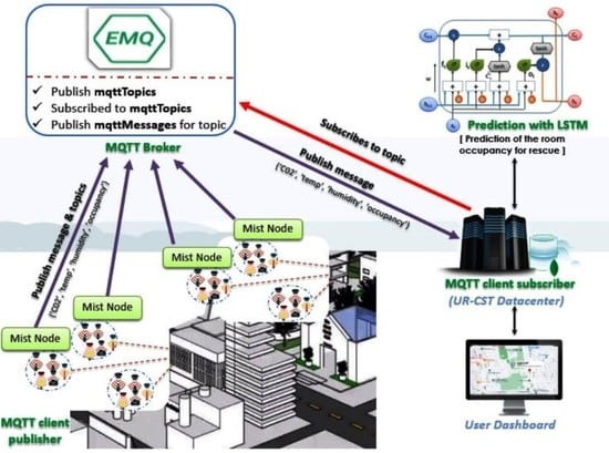
2.1. Node Layer

The conducted research had been implemented in the University of Rwanda building located in Kigali city Rwanda. The developed kit consisted of the selected sensors according to designed architecture to acquire environmental parameters to be used for further prediction. These sensors are namely temperature sensor, humidity sensor, lighting sensor, CO₂ sensor, and the passive infrared sensor also known as a motion sensor for occupant detection as listed in

Table 1. Sensors used in the development kit.

Component	Characteristics	Manufacturing
Mist node	Temperature, Humidity	Adafruit
PIR Motion	Occupancy	Adafruit
MQ-135	CO2	Adafruit
LM393 Light Detector	Light	Adafruit

. A global positioning system (GPS) is used to locate the building. Besides, all buildings with their corresponding rooms are labeled to allow precise location for the quick rescue of victims done by emergency response coordinators.

All sensor modules are connected to an ESP 8266 microcontroller NodeMCU. The NodeMCU has an inbuilt WIFI module to allow data transmission to the gateway followed on to the cloud respectively as shown in Figure 3.

Table 2. Components of the developed architecture.

Component	Characteristics
Mist node	Composed of sensors and a microcontroller Quick decision for controlling actuators Allow data access control and privacy mechanism
Fog node	Located in University of Rwanda Datacenter Allow real-time data storage Allow real-time data processing Allow real-time data monitoring
Cloud node	Uses third-party cloud services Data are sent there for public access and decision making Allow prediction analysis

describes each component used in Figure 3 with their characteristics in this research context.

The reason for choosing this architecture is to make a flexible framework to decide at any point in time based on the criticalities of the situation. In case of fire, the mist node takes a quick reaction by activating the actuators in a specific room, for example, the sprinklers act by spraying water as listed with characteristics in

Table 3. Actuators used in the development.

Component	Characteristics
Sound alarm	Senses an abnormal condition within the system. Provides a signal indicating the presence of the abnormality.
LED light	Provides light using one or more light-emitting diodes. LED lamps have a lifespan many times longer than equivalent incandescent lamps.
Sprinkler	Discharges water when the effects of a fire have been detected.

. At the fog node, all possible collected data is stored in the datacenter of the institution for real-time analysis/data processing by reducing the latency of the wide-area network. At the cloud node, third-party cloud services are selected, allowing public data access for decision-making followed by prediction analysis.

The mist node had been deployed in a selected room for 15 days. Data was transmitted using WIFI technology to the back-end server database within a one-minute time interval. The collected data are extracted into comma-separated value (CSV) format for prediction purposes.

2.2. GPS Sensor

GPS is a satellite-based radio navigation system owned by the US government and operated by the United States Space Force. GPS technology enables the use of GPS devices as navigation and orientation tools as well as instruments used to capture traveled routes [18,19]. It has been used in several sectors such as travel mode detection [20] physical activity detection [18], and for informing classifiers for detecting physical activities’ types [18,19,21].

The GPS data has composite types of parameters that are used to allocate a specific object relying on the earth. GPS data include latitude, longitude, date, time, horizontal dilution of precision, vertical dilution of precision, number of satellites, altitude, and instantaneous speed [18].

The latitude and longitude parameters captured by the GPS allow the localization of the affected building. In order to alleviate the problem of locating victims in the vertical direction, the sensor node is labeled based on the room number along with the building’s floor number indicating the deployed microcontroller.

2.3. MQTT Protocol

Message Queuing Telemetry Transport (MQTT) is an application layer protocol adopted for different applications such as monitoring data [22], user energy management [23], notification systems [24], handling mobility [25], heart and electrocardiogram monitoring [26,27], it was adopted in the past by large-scale companies like Facebook in the messenger application [28].

It is a client-server publish/subscribe messaging transport protocol. It is a lightweight, open, simple design to be easily implemented. These characteristics allow it to be used in constrained environments such as communication in the machine to machine (M2M) with IoT contexts where a small code footprint is required even if network bandwidth is at a premium [29].

Building an IoT system requires IoT data transmission using IoT communication middleware. A topic is identified by a unique string. That string represents the hierarchy of topics themselves. This is similar to how folders are identified on a computer. All information is organized on different topics. Each client connected to the broker could be either an information subscriber or publisher. As the protocol exchanges data through topics while all devices with the same topic are connected to the broker hence, its location is important for MQTT broker-based IoT middleware [30].

Every time a publisher (mist node) will post a new message on a topic (sensor data), the MQTT broker (EMQ) forwards that message to all subscribed clients (MongoDB) to that topic. In this way, publishers and subscribers could send or receive data ignoring the existence with the locations of other clients. Another important MQTT feature is the possibility of setting different Quality of Services (QoS) in client connection to the broker. A different level of QoS determines a different security level regarding the delivery of the message to the destination [31,32].

MQTT protocol has been chosen from HTTP even though they have a considerably smaller footprint. MQTT protocol is suitable for resource-constrained environments. All MQTT-based brokers have similar or comparable abilities. The Mosquito broker by default does not provide security for its messaging scheme. Here authentication information is sent in plaintext therefore, it requires security mechanisms to protect the transferred information [33].

In this context, from the available MQTT brokers explored, the two open sources (Mosquito, and Erlang MQTT) had been explored, the latter is chosen. EMQ broker provides a scalable, reliable, enterprise-grade PUB/SUB MQTT message Hub for IoT. It is written in Erlang/OTP under Apache Version 2.0 that is cross-platform, which was deployed on different operating systems and even Raspberry Pi [34]. EMQ implements both MQTT V3.1 and V3.1.1 protocol specifications and supports MQTT-SN, CoAP, WebSocket, STOMP, and SockJS at the same time [35].

In the framework displayed in Figure 4, the environmental parameters are acquired from a room, including the room name, floor number, and the geo-location of the building. This data is sent to the EMQ broker followed by the MQTT client subscriber as shown in Figure 4.

2.4. Data Storage

Mongo is an open-source schemaless, Not Only SQL (NoSQL), document-based database that stores and retrieves documents as extensive Markup language (XML), JavaScript Object Notification (JSON), binary JSON (BSON) [36]. New techniques in the database context have evolved towards NoSQL [37]. In this research, Mongo is selected as it can support the variety, volume, and velocity features of Big Data. The system implemented with Mongo, includes horizontal scalability, linearization, high availability, and fault tolerance. The database server is responsible for recording room physical environmental parameters every 1 min resulting in a huge amount of data. The retrieval is simple for the different real-time user interfaces.

2.5. Prediction Model Based on LSTM

Recurrent Neural Network (RNN) methods are a special type of neural network designed for sequence problems. They have been used to create sequential information data for deep learning applications such as object tracking [38], image classification [39], speech recognition [40], and language translation [41]. One of the RNN types is LSTM. LSTM overcomes the limitations of RNN with the lack of full information on how to train the network with backpropagation. It also enables to stop gradients from vanishing or exploding during training.

A common LSTM unit shown in Figure 5 is composed of a cell, an input gate, forget gate, and an output gate. The cell remembers values over arbitrary time intervals. The three gates regulate the flow of information into and out of the cell.

The LSTM cell as shown in Figure 6 is composed of inputs, outputs, vector operators, and nonlinearities are responsible for kee** track of the dependencies between the elements in the input sequence. The input gate denoted by it controls the extent to which a new value flows into the cell. The forget gate controls the extent to which a value remains in the cell. The output gate denoted by O_t controls the extent to which the value in the cell is used to compute the output activation of the LSTM unit. The candidate gate denoted by Č_t controls what data to write to the cell state.

The inputs are of three types. The first is C_t−1 that indicates memory from the previous/last LSTM unit. The second is h_t−1 that indicates the output state of the previous/last LSTM unit. The third is X_t indicating the current input. The outputs are of two types. The first is C_t that indicates new updated memory. The second is h_t that indicates the current output state. The vector operations are of two types. The first is x indicates the scaling of information while the second + indicates adding information. The nonlinearities are of two-three types. The first one is the sigmoid layer denoted by σ. The second is tanh layer is denoted by tanh. The third is the bias denoted by bi.

The activation function of the LSTM gates is often a logistic sigmoid function denoted by σ. There are connections into and out of the LSTM gates, a few of which are recurrent. The weights of these connections that need to be learned during the training of the model determine how the four gates inter-operate.

The first step in LSTM is to decide the information that needs to be discarded away from the cell state. This decision is made by a sigmoid layer called the forget gate layer. It takes h_t−1 and X_t, and outputs a number between 0 and 1 for each number in the cell state C_t−1. Here, 1 represents to keep it while 0 represents to discard it.

The next step is to decide the new information to be stored in the cell state. This has two parts. First, a sigmoid layer called the input gate layer decides the values to be updated. Next, a tanh layer creates a vector of new candidate values, Č_t, which could be added to the state. The next step is to combine it and Č_t to create an update to the state.

The next step is to update the old cell state, C_t−1, into the new cell state C_t. In order to obtain a new cell state Ct, the old state is multiplied by ft, forgetting the things decided to be forgotten earlier. Then add it ∗ Č_t. These are the new candidate values, scaled to update each state value.

This output will be based on the cell state but will be a filtered version. The sigmoid layer decides the parts of the cell state to output. Then the cell state is put through tanh (to push the values to be between −1 and 1) and multiply it by the output of the sigmoid gate so that the decoded output is achieved.

The operator ⊙ presented in the formula for C_t and ht denotes element-wise multiplication (labeled as the scaling of information in the diagram with multiplication symbol as shown in Figure 6). Thus, the output at each time step depends on previous inputs and past computation.

In the context of occupancy prediction from the acquired data as the research is proposing the use of multivariate features, the input of data features is denoted as $Xi=\left(x1, x2, x3, x4, x5\right)$ where 1, 2, 3, 4, and 5 represent temperature, humidity, CO₂, occupancy, and date respectively. The hidden state of memory block $h=\left(h1, h2, h3, ..\right)$, depends on the number of LSTM state network used with the real output sequence $O=\left(o1, o2\right)$ (where 1 and 2 denote occupant and time respectively) are being iteratively calculated by the equations mentioned in Figure 6. In case the data needs iteration bias is added.

Series Prediction with LSTM Neural Network

In the context of environmental time-series data, the prediction process, the construction of an LSTM neural network shown in Figure 6 using the LSTM series of the cell is unfolded in Figure 7. At time t − 1, the input of the network is the observed historical data X_t−1 and the output is the predicted future data where X is the observed occupancy time sequence.

Figure 7 describes the series of LSTM gates to construct the prediction architecture.

3. Results

3.1. Data Acquisition

In the experimental setup configuration, the developed system including humidity, temperature, CO₂, light, and proximity sensors is implemented in a working office, located in the University of Rwanda, KARISIMBI Building for around 15 days. The sensors are connected to an ESP8266 microcontroller board with its WIFI module enabled to send data to the local configured MongoDB database server. The selected indoor environmental parameters are considered by different researchers to detect the presence of human beings. However, the key additional parameter is the use of a proximity sensor to detect any human presence along with the other captured variables. The geo-location information is captured to allow localization of the victims in case of a fire or any incidences that occur. The output of the system displays on the web interface linked to the google map of the experimented building location.

The presence of human beings is indicated by the increase of CO₂ as it is the gas produced during exhalation [42]. The other is used to infer the knowledge of human presence in a specific room also. The experiment did not consider the windows open or closed which can reduce the amount of CO₂ concentration in the room. The position of the kit was centered in the room. The room is a shared room with a proximity sensor is placed near the door to capture any movement of humans.

Figure 8 shows the developed system in its operational mode during the testing phase. The data are sent to the back-end database in 1-minute time interval to avoid redundancy of similar records. Figure 9b shows the close-up of sensor node localization on the google map with minimum average parameters.

3.2. Preparation of Data for Multivariate Forecast Model

The time series acquired data from the experiment to the gateway server are converted to CSV format to be used in LSTM as input data. Before LSTM data preparation in Anaconda Python, a separate environment is created by the installation of Keras with Theano, as TensorFlow proved the slowness of the system used for implementation. Scikit-learn, Pandas, NumPy, Seaborn, and Matplotlib libraries are also installed for data preprocessing, visualization, and machine learning algorithms. Preprocessing of the data was conducted as an initial phase for the prediction that is required for missing values tracking and elimination. At this step, the time-series data is to fill the missed values. The interpolation of the variables before and after a timestamp is used for missed values. Figure 10 shows the sample of the first five rows retrieved using head() method in pandas among 19,879 records of the dataset.

3.3. Collinearity of the Data

In the assessment of the correlation between the variables for better prediction, the collinearity is computed to check how they are associated with each other. In this operation, the heatmap function of the seaborn library of python is used. Figure 10 shows how data are correlated for selected Karisimbi building in the experimental office omitting some variables (geo-location data).

Figure 11a some parameters are correlated in the sense that gives an insight into their relationship. The full correlated data has a value of 1, while the worse correlated data has around zero value. The acquired data shows an obvious correlation between the occupancy variable and the light data. Moreover, there is a better correlation between occupancy with CO₂ and Temperature parameters respectively. Figure 11b describes how all parameters are related to occupancy data.

3.4. Data Preparation for LSTM Model

The occupancy dataset preparation for the LSTM model must be framed as a supervised learning problem. The data are multivariate data that require input variables to be normalized [43]. The data set is composed of multiple variables of different units. The reason for the re-scaling technique to be used as a normalization technique to stretch and squeeze the values in the datasets to fit on a scale from 0 to 1. The model setup is considered to predict the occupancy at the next hours from the previous measurements at the prior time steps of five input variables used [temperature, humidity, light, occupancy, and CO₂] in the experiment. The dataset is split into two parts that are train and test sets with 70% and 30% respectively. Then the train and test are split into input and output variables. The LSTM model expects 3D dimension variables namely [samples, timesteps, features] reshaped from input variables. Different configurations are done progressively, which is to define the first hidden layer with 1 neuron for predicting occupancy. The input shape will be a 3-times step with 5 features. The efficient Adam version of stochastic gradient descent is used with the Mean Squared Error (MSE) loss function. This research used 50 training epochs with a batch size of 64 of four iterations for a better fit model. The authors explored the appropriateness justification of deep learning towards the usage of automatic feature extraction. The adoption of real-time experimental data is something that was inspired to adopt in this research future work [44]. The importance of multivariate or multimodal data has been explored [45]. The authors register the point that most research articles have still explored time sequence data mostly. So, this paper with the application area of air pollution prediction has explored generative adversarial networks along with data augmentation through raw images to overcome the class imbalance. This has shown considerable improvement in classification accuracy.

3.5. Training Results

The learning process for the recurrent neural network that uses Long Short-Term Memory (LSTM) cells is configured as an iterative process of the optimization of the weights. The weights are updated in each epoch. Once the training starts, the aim is to generate predictions by minimizing the loss function. The performance of the network is then evaluated on the test set. The training process ends when the error on the validation set begins to increase as this could mark the beginning of a phase of overfitting the data.

The model training and validation loss of the implemented LSTM recurrent neural network is presented in Figure 12. The observation shows that as the number of epochs increases the training model becomes the best fit.

3.6. Performance Metrics

In this research paper, the evaluation of the experiment conducted using Naïve Bayes Classifier, SVM, and Multilayer Perceptron Feed-Forward Network against LSTM, which is one of RNN method- LSTM for occupancy prediction. In each experiment, the results were assessed by the following evaluation measures such as root square score, mean absolute error, root means squared error, accuracy, and standard deviation. The modeling scenario used in this research is considered as a regression problem that is a set of statistical processes for estimating the relationships between a dependent variable (often called the outcome variable) and one or more independent variables (often called predictors, covariates, or features).

3.6.1. Root Square Score (R²)

The performance metric of the model is evaluated using a root squared score. It is the coefficient of determination [46], that represents the proportion of variance that has been explained by the independent variables in the model. It provides an indication of goodness of fit and therefore a measure of how well-unseen samples are likely to be predicted by the model through the proportion of explained variance. The metric has crucial importance in measuring the efficiency of the model that means that its values range from zero to one [0, 1]. Here zero (0) illustrates that the proposed model does not improve the prediction over the mean model while one (1) implies the perfect prediction.

If $\widehat{y_i}$ is the predicted value of the ith sample and $y_i$ is the corresponding true value for the total n sample, the estimated R² is defined as follows.

$$R^2\left(y,\widehat{y}\right)=1-\frac{{{\displaystyle \sum }}_{i=0}^n{\left(y_i-{\widehat{y}}_i\right)}^2}{{{\displaystyle \sum }}_{i=0}^n{\left(y_i-{\overline{y}}_i\right)}^2}$$

(1)

3.6.2. Mean Absolute Error (MAE)

The mean absolute error is a risk metric corresponding to the expected value of the absolute error loss. It measures the distinguished values between two continuous variables [47]. If $\widehat{y_i}$ is the predicted value of the ith sample and $y_i$ is the corresponding true value for total $n$ sample, then the mean absolute error (MAE) estimated over $n$ samples is defined as follow.

$$MAE\left(y,\widehat{y}\right)=\frac{1}{n}{{\displaystyle \sum }}_{i=0}^{n-1}\left|y_i-{\widehat{y}}_i\right|$$

(2)

3.6.3. Root Mean Squared Error (RMSE)

The Root Mean Square Error (RMSE) is the standard deviation of the residuals (prediction errors). Residuals are a measure of how far from the regression line data points are; RMSE is a measure of how spread-out these residuals are [48]. In other words, it says that the concentrated data is around the line of best fit. Root mean square error is commonly used in many sectors for experimental results verifications [44]. A framework capable of solar power forecasting in a smart grid is proposed [49]. It is achieved through Autoregression (univariate) framework and the optimization is achieved through RMSE. They are yet to explore multivariate that will help support better smart grit management by incorporating information from smart meters and other electronic devices. In this proposed work, the incorporation of multivariate data analysis was done for better result accuracy.

If $\widehat{y_i}$ is the predicted value of the ith sample and $y_i$ is the corresponding true value for the total $n$ sample, then the root mean squared error (RMSE) estimated over $n$ samples is defined as follows.

$$RMSE\left(y,\widehat{y}\right)=\sqrt{\frac{1}{n}{{\displaystyle \sum }}_{i=0}^{n-1}{\left(y_i-{\widehat{y}}_i\right)}^2}$$

(3)

3.6.4. Standard Deviation (SD)

It is the measure of the dispersion of statistical data. Dispersion computes the deviation of data from its mean of average position. A large standard deviation indicates that the data points can spread from the mean and a small standard deviation indicates that they are clustered closely around the mean.

Let the sample size be n with a mean of $\overline{Y}$, the standard deviation (SD) is calculated using the following equation:

$$SD=\sqrt{\frac{1}{n}{{\displaystyle \sum }}_{i=0}^{n-1}{\left|y_i-\overline{Y}\right|}^2}$$

(4)

These performance measures give the indicators for the determination of the effectiveness of the model for forecasting the daily stock index [50,51,52]. The standard deviation has been well used in [53] for multivariate time series in smart grids.

A new forecasting model claimed to outperform conventional autoregression and vector autoregression models is proposed [54]. This was made possible by incorporating the least absolute shrinkage and selection operator (LASSO) framework, as the case study involves sparse placements of wind power. This paper has inspired our future work when we are planning to expand the work across various places in the cities of Rwanda. The importance of Spatio-temporal autocorrelation arrived from various data sources will be added advantage to avoid inaccurate predictions [55]. The application explored is the energy domain, as mostly in these domains many papers have usually explored only temporal data. This work is reflected in this current research work through the adoption of Spatio-temporal data in our data set.

The change detection in the application that involves streaming data is significantly described [53]. The approach has improved the quality of results by overcoming false positive detection, additional changes in new incoming data. The paper will be crucial in our future enhancement when deployed across cities, which creates the possibility for more and more new data, whereby the training and test datasets need to be rewired accordingly.

3.7. Comparative Analysis of Machine Learning Results

The results of the LSTM model are compared to two machine learning algorithms and one deep learning algorithm tested against the same dataset to evaluate the efficiency of the proposed model. In the selected model to compare the obtained errors, the minimum model loss that is attained on the hyperparameter values is shown in

Table 4. Model parameters optimal values in the experiment.

Parameter	Optimal Model Values for Occupancy Dataset
Train dataset lot	70%
Test dataset lot	30%
Input layer	1
LSTM cells	2 cells
Activation function	Rectified Linear Unit (ReLu)
Dropout wrapper	0.4
Dense Layer	1
Optimizer	Adam
Number of Epochs	50
Batch size	100
Look back window	8
Loss function	MAE

.

Table 5. Performance measure values.

Approaches	Accuracy	MAE	RMSE	R2	SD
LSTM	0.968	0.02317	0.08397	0.9566	0.347
Naïve Bayes Classifier	0.867	0.13294	0.36461	0.0908	0.4626
Support Vector Machine	0.822	0.17785	0.42172	−0.2163	0.0000
Multilayer Perceptron FFN	0967	0.03193	0.17871	0.7815	0.44669

presented the experimental results.

Figure 12 shows the training and test loss of the proposed LSTM model at optimal parameters values described in Table 4. The diagrams show that the train and test losses decrease for larger epoch values and that train as well as test losses both stabilize at closer points. The loss instability in the occupant model resulted from data complexity due to the continuous changes of light intensity during one or more combinations of the daylight or/and the windows open.

Figure 13 describes the actual and predicted values of the selected parameters such as temperature, humidity, CO_2, and light from the LSTM model described in Figure 6. As shown on the legends the true values are in orange while the predicted values are in blue.

Table 5 presents the comparative minimum error values as well as model performance accuracy of the proposed model with other models (Naïve Bayes Classifier, Support Vector Machine, and Multilayer Perceptron Feed Forward Network). The results show that LSTM has a high accuracy compared to other models and the error values are minimized in comparison to them.

Figure 14 presents the result showing that LSTM performs well compared to other methods.

In Figure 14, the LSTM network presents better performance than the other selected algorithms namely, Naïve Bayes, Support Vector Machine, and Multilayer Perceptron Feed-Forward Network in all error measures. The predicted RMSE of those compared machine learning algorithms is 0.36, 0.42, and 0.17 respectively, while the predicted RMSE of the proposed model is 0.083. The prediction result of those compared machine learning algorithms enhances by 77.57%, 80%, and 53.37% respectively compared to the deep learning recurrent neuron network LSTM model. While the root means squared error (R²) of the LSTM model is 96% indicating to be amongst the best. The support vector machine algorithm is showing the worse results that seem like it is not responding to the data set parameters used in this research. Multilayer Perceptron FFN results are presentable with its accuracy almost similar to LSTM as both algorithms for deep learning algorithms use a feed-forward network to train the data. The Standard deviation comparisons also confirm LSTM to provide the least deviated predicted values.

4. Discussion

This research paper implements a method for an IoT-based framework to collect environmental indoor room parameter-based multivariate time-series data to be uploaded on the central gateway database using MQTT protocol as shown in Figure 3. The collected data was analyzed by deep learning algorithms for the presence of human beings to be rescued from the building. This is to inform the fire brigade of the location of the presence of human beings in a building. Comparative analysis of deep learning algorithms was also conducted with error measurement techniques.

The reason for choosing MQTT over HTTP communication protocol is to allow real-time data ingestion into the database as HTTP protocol considered as client/server presents a communication overhead. The system was configured in the publish-subscribe paradigm in such a way that sent parameters are considered as topics and the continuous sent data are considered as messages, in another word it is topic/message policy as shown in Figure 4. The configuration of the mist node is an MQTT-client publisher to the MQTT-broker with the role of publishing data to the broker. The database is configured as an MQTT-client subscriber to be precise.

The messages acquired from the mist node are collected to the gateway server database as shown in Figure 4. In this research a no-relational database management system MongoDB is used, which allows scalability, and replication. The API (web services) was developed to read data from the database to display them to the user interface as shown in Figure 9b. The experimental setup is tested for 15 days and the data are saved within a 1-min time interval to a time series data set as shown in Figure 9a.

The time-series data collected is exported in CSV format for further processing in the next phase as shown in Figure 10. The research paper developed a method to predict room occupancy using deep learning-based methodology as a regression problem. All parameters are analyzed by considering the correlation between each variable to explore the possibility of inferring the knowledge as shown in Figure 11. The modeled data were considered as multivariate multi-step time series data. The background of machine learning techniques used in this research paper explored the techniques that model the real-time collected data efficiently with LSTM as shown in Figure 6 predicting the best accuracy amongst all chosen as shown in Table 5.

In particular, LSTM shows to over-perform the widely used machine learning algorithms such as Naïve Bayes and Support Vector Machines model. The implemented LSTM model is compared with another deep learning algorithm such as Multilayer Perceptron Feed Forward Network that confirms a reasonable result compared to the other machine learning techniques as shown in Figure 14.

In conclusion, the proposed LSTM model using captured real-time collected data is compared for performance metrics with other algorithms as shown in Figure 14. The LSTM model’s accuracy is 96% on the tested multivariate captured data that is nearly 16% better than the best of the others. The LSTM model does not over-fit from the used data and minimizes the loss that can infer their prediction.

The various limitations in this research use different parameters such as temperature, humidity, light, humidity ratio, and occupancy as data to predict the presence of an occupant within the room. A lot of observations had been explored as limitations of variables or biases to affect the prediction results. CO₂, pressure, and humidity parameters were reported to be noisy when the experimental setup is not conducted in a controlled environment hence, it brought unconvincing prediction results.

Research also shows that the light parameter can be noisy too due to daylight differentiation. While other researchers used dust sensors, noise sensors, and cameras to have a precise prediction, it is also shown that dust, noise can be interrupted by other external and internal factors like dragging of chairs and so on. Data captured by the camera shows that they can expose privacy thus currently eliminated from the discussion.

This research took advantage of a mixture of different parameters as multivariate data in the prediction models instead of univariate data for each parameter among temperature, humidity, light, humidity ratio, and occupancy to enhance the experimental accuracy of the models.

In future research, the consideration of collecting data from additional similar enclosed environments using deployed IoT sensor kit at various places across cities of Rwanda will be taken care of. Further, the FIWARE, an open-source platform for smart environments will be explored. Moreover, the temporal dependence of data on the occupancy level should be examined. Besides, the impact of external factors (weather conditions, noise, and airflow) on the prediction accuracy should be considered. The extension of both univariant and multivariant data with Noise-canceling/avoiding techniques to precisely measure real-time prediction models with even better accuracy is also planned. Furthermore, we will explore how the deeper layers of LSTM could affect the performance of the model concerning the tested multivariate time series data set. Finally, further evaluations with other more deep-learning models will be performed to investigate the gates that have the most influential role.

References

1. Stamford, C. Analysts to Explore the Value and Impact of IoT on Business at Gartner. 2015. Available online: https://www.gartner.com/en/newsroom/press-releases/2015-11-10-gartner-says-6-billion-connected-things-will-be-in-use-in-2016-up-30-percent-from-2015 (accessed on 17 July 2020).
2. Ahmad, S.; Kim, D. Design and implementation of thermal comfort system based on tasks allocation mechanism in smart homes. Sustainability 2019, 11, 5849. [Google Scholar]
3. Park, H.; Rhee, S.B. IoT-Based Smart Building Environment Service for Occupants’ Thermal Comfort. Available online: https://www.hindawi.com/journals/js/2018/1757409/ (accessed on 5 January 2020).
4. East African Community. Disaster Risk Reduction and Management Strategy (2012–2016). Available online: https://www.ifrc.org/Global/Publications/IDRL/regional/EAC_DRRMS(2012-2016).pdf (accessed on 6 January 2020).
5. The Republic of Rwanda, Ministry in Charge of Emergency Management. Available online: https://www.minema.gov.rw/fileadmin/user_upload/Minema/Publications/Contingency_Plans/Contingency_Plan_for_Fire_Incidents.pdf (accessed on 8 January 2020).
6. Republic of Rwanda; Ministry of Infrastructure, Urbanization and Rural Settlement. Available online: http://www.minecofin.gov.rw/fileadmin/templates/documents/NDPR/Sector_Strategic_Plans/Urbanization_and_Rural_Settlement.pdf (accessed on 7 January 2020).
7. Bettin, G.; Zazzaro, A. The Impact of Natural Disasters on Remittances to Low- and Middle-income Countries. Dev. Work. Pap. 2016, 54, 481–500. [Google Scholar] [CrossRef] [Green Version]
8. Mondal, D.R. High Risk of Post-Earthquake Fire Hazard in Dhaka, Bangladesh. Fire 2019, 2, 24. [Google Scholar] [CrossRef] [Green Version]
9. Lam, H.C.Y.; Haines, A.; McGregor, G.; Chan, E.Y.Y.; Hajat, S. Time-Series Study of Associations between Rates of People Affected by Disasters and the El Niño Southern Oscillation (ENSO) Cycle. Int. J. Environ. Res. Public Health 2019, 16, 3146. [Google Scholar] [CrossRef] [Green Version]
10. Ghai, S.K.; Thanayankizil, L.V.; Seetharam, D.P.; Chakraborty, D. Occupancy detection in commercial buildings using opportunistic context sources. In Proceedings of the 2012 IEEE International Conference on Pervasive Computing and Communications Workshops, Lugano, Switzerland, 19–23 May 2012. [Google Scholar]
11. Zikos, S.; Tsolakis, A.; Meskos, D.; Tryferidis, A.; Tzovaras, D. Conditional Random Fields—Based approach for real-time building occupancy estimation with multi-sensory networks. Autom. Constr. 2016, 68, 128–145. [Google Scholar] [CrossRef]
12. Dey, A.; Ling, X.; Syed, A.; Zheng, Y.; Landowski, B.; Anderson, D.; Stuart, K.; Tolentino, M.E. Namatad: Inferring occupancy from building sensors using machine learning. In Proceedings of the 2016 IEEE 3rd World Forum Internet Things, Reston, VA, USA, 12–14 December 2016. [Google Scholar]
13. Xayasouk, T.; Lee, H.M.; Lee, G. Air pollution prediction using long short-term memory (LSTM) and deep autoencoder (DAE) models. Sustainability 2020, 12, 2570. [Google Scholar] [CrossRef] [Green Version]
14. Le, X.H.; Ho, H.V.; Lee, G.; Jung, S. Application of Long Short-Term Memory (LSTM) neural network for flood forecasting. Water 2019, 11, 1387. [Google Scholar] [CrossRef] [Green Version]
15. Zhao, Z.; Chen, W.; Wu, X.; Chen, P.C.V.; Liu, J. LSTM network: A deep learning approach for short-term traffic forecast. IET Image Process. 2017, 11, 68–75. [Google Scholar] [CrossRef] [Green Version]
16. Choi, E.; Cho, S.; Kim, D.K. Power demand forecasting using long short-term memory (LSTM) deep-learning model for monitoring energy sustainability. Sustainability 2020, 12, 1109. [Google Scholar] [CrossRef] [Green Version]
17. Liu, P.; Wang, J.; Sangaiah, A.; **e, Y.; Yin, X. Analysis and Prediction of Water Quality Using LSTM Deep Neural Networks in IoT Environment. Sustainability 2019, 11, 2058. [Google Scholar] [CrossRef] [Green Version]
18. Allahbakhshi, H.; Conrow, L.; Naimi, B.; Weibel, R. Using accelerometer and GPS data for real-life physical activity type detection. Sensors 2020, 20, 588. [Google Scholar] [CrossRef] [Green Version]
19. Almanza, E.; Jerrett, M.; Dunton, G.; Seto, E.; Pentz, M.A. A study of community design, greenness, and physical activity in children using satellite, GPS and accelerometer data. Health Place 2012, 18, 46–54. [Google Scholar] [CrossRef] [Green Version]
20. Wu, L.; Yang, B.; **g, P. Travel Mode Detection Based on GPS Raw Data Collected by Smartphones: A Systematic Review of the Existing Methodologies. Information 2016, 7, 67. [Google Scholar] [CrossRef] [Green Version]
21. Miller, H.J.; Tribby, C.P.; Brown, B.B.; Smith, K.R.; Werner, C.M.; Wolf, J.; Wilson, L.B.; Oliveira, M.G.S. Public transit generates new physical activity: Evidence from individual GPS and accelerometer data before and after light rail construction in a neighborhood of Salt Lake City, Utah, USA. Health Place 2015, 36, 8–17. [Google Scholar] [CrossRef] [Green Version]
22. Grgić, K.; Špeh, I.; Heđi, I. A web-based IoT solution for monitoring data using MQTT protocol. In Proceedings of 2016 International Conference on Smart Systems and Technologies, Osijek, Croatia, 12–14 October 2016; pp. 249–253. [Google Scholar]
23. Jia, K.; **ao, J.; Fan, S.; He, G. An MQTT/MQTT-SN-Based User Energy Management System for Automated Residential Demand Response: Formal Verification and Cyber-Physical Performance Evaluation. Appl. Sci. 2018, 8, 1035. [Google Scholar] [CrossRef] [Green Version]
24. Tang, K.; Wang, Y.; Liu, H.; Sheng, Y.; Wang, X.; Wei, Z. Design and Implementation of Push Notification System Based on the MQTT Protocol. In Proceedings of the 2013 International Conference on Information Science and Computer Applications (ISCA 2013); Atlantis Press: Amsterdam, The Netherlands, 2013; pp. 116–119. [Google Scholar]
25. Luzuriaga, J.E.; Cano, J.C.; Calafate, C.; Manzoni, P.; Perez, M.; Boronat, P. Handling mobility in IoT applications using the MQTT protocol. In Proceedings of the 2015 Internet Technologies and Applications, ITA 2015—Proceedings of the 6th International Conference, Wrexham, UK, 8–11 September 2015; Institute of Electrical and Electronics Engineers (IEEE): New York City, NY, USA, 2015; pp. 245–250. [Google Scholar]
26. Barata, D.; Louzada, G.; Carreiro, A.; Damasceno, A. System of Acquisition, Transmission, Storage and Visualization of Pulse Oximeter and ECG Data Using Android and MQTT. Procedia Technol. 2013, 9, 1265–1272. [Google Scholar] [CrossRef]
27. Chooruang, K.; Mangkalakeeree, P. Wireless Heart Rate Monitoring System Using MQTT. Procedia Comput. Sci. 2016, 86, 160–163. [Google Scholar] [CrossRef] [Green Version]
28. Lee, S.; Kim, H.; Hong, D.K.; Ju, H. Correlation analysis of MQTT loss and delay according to QoS level. In International Conference on Information Networking; IEEE: New York City, NY, USA, 2013; pp. 714–717. [Google Scholar]
29. OASIS Standard Incorporating Approved Errata 01 | StandICT.eu. Available online: https://www.standict.eu/standards-watch/oasis-standard-incorporating-approved-errata-01 (accessed on 20 July 2020).
30. Govindan, K.; Azad, A.P. End-to-end service assurance in IoT MQTT-SN. In Proceedings of the 2015 12th Annual IEEE Consumer Communications and Networking Conference, CCNC, Las Vegas, NV, USA, 9–12 January 2015; Volume 2015, pp. 290–296. [Google Scholar]
31. Vafeiadis, T.; Zikos, S.; Stavropoulos, G.; Ioannidis, D.; Krinidis, S.; Tzovaras, D.; Moustakas, K. Machine Learning Based Occupancy Detection Via The Use of Smart Meters. 2017. Available online: https://www.encompass-project.eu/wp-content/uploads/2017/10/ICESEE17_occupancy.pdf (accessed on 31 January 2021).
32. Cesana, M.; Redondi, A.; Longo, E.; Giardini, G. Machine Learning Methods for Indoor Occupancy Detection with CO2 Multi-sensor Data. Available online: https://www.politesi.polimi.it/bitstream/10589/147394/3/Tesi_Giorgio_Giardini_874841.pdf (accessed on 21 July 2020).
33. Dinculeană, D.; Cheng, X. Vulnerabilities and Limitations of MQTT Protocol Used between IoT Devices. Appl. Sci. 2019, 9, 848. [Google Scholar] [CrossRef] [Green Version]
34. Sánchez, P.; Álvarez, B.; Antolinos, E.; Fernández, D.; Iborra, A. A teleo-reactive node for implementing internet of things systems. Sensors 2018, 18, 1059. [Google Scholar] [CrossRef] [Green Version]
35. EMQ—Erlang MQTT Broker—EMQ 2.2—Erlang MQTT Broker 2.2-beta.1 Documentation. Available online: https://docs.emqx.io/broker/v2/en/index.html (accessed on 20 July 2020).
36. Kaur, K.; Rani, R. Modeling and querying data in NoSQL databases. In Proceedings—2013 IEEE International Conference on Big Data, Big Data; IEEE: New York City, NY, USA, 2013; Volume 2013, pp. 1–7. [Google Scholar]
37. Martinez-Mosquera, D.; Navarrete, R.; Lujan-Mora, S. Modeling and management big data in the databases—A systematic literature review. Sustainability 2020, 12, 634. [Google Scholar] [CrossRef] [Green Version]
38. Milan, A.; Rezatofighi, S.H.; Dick, A.; Reid, I.; Schindler, K. Online Multi-Target Tracking Using Recurrent Neural Networks. In Proceedings of the AAAI Conference on Artificial Intelligence, San Francisco, CA, USA, 4–9 February 2017. [Google Scholar]
39. Wang, Q.; Lin, J.; Yuan, Y. Salient Band Selection for Hyperspectral Image Classification via Manifold Ranking. IEEE Trans. Neural Netw. Learn. Syst. 2016, 27, 1279–1289. [Google Scholar] [CrossRef]
40. Graves, A.; Mohamed, A.; Hinton, G. Speech Recognition with Deep Recurrent Neural Networks. In ICASSP, 2013 IEEE International Conference on Acoustics, Speech and Signal Processing; IEEE: New York City, NY, USA, 2013; pp. 6645–6649. [Google Scholar]
41. Mahata, S.K.; Das, D.; Bandyopadhyay, S. MTIL2017: Machine translation using recurrent neural network on statistical machine translation. J. Intell. Syst. 2019, 28, 447–453. [Google Scholar] [CrossRef] [Green Version]
42. Vedantu Learn LIVE Online, NCERT—National Council of Educational Research and Training. Available online: https://www.vedantu.com/ncert-solutions/ncert-solutions-class-11-biology-chapter-17-breathing-and-exchange-of-gases (accessed on 8 June 2020).
43. How to Diagnose Overfitting and Underfitting of LSTM Models. Available online: https://machinelearningmastery.com/diagnose-overfitting-underfitting-lstm-models/ (accessed on 30 September 2020).
44. Georgakopoulos, S.V.; Tasoulis, S.K.; Mallis, G.I.; Vrahatis, A.G.; Plagianakos, V.P.; Maglogiannis, I.G. Change detection and convolution neural networks for fall recognition. Neural Comput. Appl. 2020, 32, 17245–17258. [Google Scholar] [CrossRef]
45. Kalajdjieski, J.; Zdravevski, E.; Corizzo, R.; Lameski, P.; Kalajdziski, S.; Pires, I.M.; Garcia, N.M.; Trajkovik, V. Air pollution prediction with multi-modal data and deep neural networks. Remote Sens. 2020, 12, 4142. [Google Scholar] [CrossRef]
46. Dufour, J. Coefficients of Determination; McGill University: Montreal, QC, Canada, 2011. [Google Scholar]
47. Chai, T.; Draxler, R.R. Root mean square error (RMSE) or mean absolute error (MAE)?-Arguments against avoiding RMSE in the literature. Geosci. Model Dev. 2014, 7, 1247–1250. [Google Scholar] [CrossRef] [Green Version]
48. RMSE: Root Mean Square Error—Statistics How to. Available online: https://www.statisticshowto.com/probability-and-statistics/regression-analysis/rmse-root-mean-square-error/ (accessed on 18 October 2020).
49. Bessa, R.J.; Trindade, A.; Silva, C.S.P.; Miranda, V. Probabilistic solar power forecasting in smart grids using distributed information. Int. J. Electr. Power Energy Syst. 2015, 72, 16–23. [Google Scholar] [CrossRef] [Green Version]
50. Chen, Y.; Abraham, A.; Yang, J.; Yang, B. Hybrid Methods for Stock Index Modeling. Available online: https://link.springer.com/chapter/10.1007/11540007_137 (accessed on 16 June 2020).
51. Lei, L. Wavelet Neural Network Prediction Method of Stock Price Trend Based on Rough Set Attribute Reduction. Appl. Soft Comput. J. 2018, 62, 923–932. [Google Scholar] [CrossRef]
52. Enke, D.; Mehdiyev, N. Stock Market Prediction Using a Combination of Stepwise Regression Analysis, Differential Evolution-based Fuzzy Clustering, and a Fuzzy Inference Neural Network. Intell. Autom. Soft Comput. 2013, 19, 636–648. [Google Scholar] [CrossRef]
53. Ceci, M.; Corizzo, R.; Japkowicz, N.; Mignone, P.; Pio, G. ECHAD: Embedding-Based Change Detection from Multivariate Time Series in Smart Grids. IEEE Access 2020, 8, 156053–156066. [Google Scholar] [CrossRef]
54. Akay, B.; Ragni, D.; Ferreira, C.S.; van Bussel, G.J.W. Investigation of the root flow in a Horizontal Axis. Wind Energy 2013, 2016, 1–20. [Google Scholar]
55. Corizzo, R.; Ceci, M.; Fanaee-T, H.; Gama, J. Multi-aspect renewable energy forecasting. Inf. Sci. 2021, 546, 701–722. [Google Scholar] [CrossRef]
Figure 1. Map of Rwanda focusing on types of urban settlements with spatial structure [6].
Futureinternet 13 00067 g001
Figure 2. Fire damages in Rwanda in the last 9 years.
Futureinternet 13 00067 g002
Figure 3. Proposed Architecture of Data Gathering.
Futureinternet 13 00067 g003
Figure 4. The proposed framework for data acquisitions and prediction mechanism.
Futureinternet 13 00067 g004
Figure 5. Common LSTM unit without details.
Futureinternet 13 00067 g005
Figure 6. LSTM cell gate complexity.
Futureinternet 13 00067 g006
Figure 7. The structure of series prediction LSTM neural network.
Futureinternet 13 00067 g007
Figure 8. (a) Prototy** setting up for data acquisition. (b) Closeup side of the data acquisition system.
Futureinternet 13 00067 g008
Figure 9. (a) Sample of captured data appealing on MongoDB user interface. (b) Close-up geographical location map of the sensor node placement with some parameters omitted.
Futureinternet 13 00067 g009
Figure 10. Sample captured data in a selected room.
Futureinternet 13 00067 g010
Figure 11. Relationship between variables: (a) Showing the collinearity of the data set; (b) Describing the pairplot of the data set used.
Futureinternet 13 00067 g011
Figure 12. LSTM model training versus test loss graph: (a) showing the training model with 8 epochs, (b) showing the training model with 50 epochs.
Futureinternet 13 00067 g012
Figure 13. Actual and predicted results: (a) for temperature, (b) for humidity, (c) for CO2, and (d) for light models.
Futureinternet 13 00067 g013
Figure 14. Prediction results: Comparative analysis of LSTM with Naïve Bayes Classifier, Support Vector Machine, and Multilayer Perceptron Feed Forward Network.
Futureinternet 13 00067 g014