Multitemporal Chlorophyll Map** in Pome Fruit Orchards from Remotely Piloted Aircraft Systems

Abstract

Early and precise spatio-temporal monitoring of tree vitality is key for steering management decisions in pome fruit orchards. Spaceborne remote sensing instruments face a tradeoff between spatial and spectral resolution, while manned aircraft sensor-platform systems are very expensive. In order to address the shortcomings of these platforms, this study investigates the potential of Remotely Piloted Aircraft Systems (RPAS) to facilitate rapid, low cost, and flexible chlorophyll monitoring. Due to the complexity of orchard scenery a robust chlorophyll retrieval model on RPAS level has not yet been developed. In this study, specific focus therefore lies on evaluating the sensitivity of retrieval models to confounding factors. For this study, multispectral and hyperspectral imagery was collected over pome fruit orchards. Sensitivities of both univariate and multivariate retrieval models were demonstrated under different species, phenology, shade, and illumination scenes. Results illustrate that multivariate models have a significantly higher accuracy than univariate models as the former provide accuracies for the canopy chlorophyll content retrieval of R² = 0.80 and Relative Root Mean Square Error (RRMSE) = 12% for the hyperspectral sensor. Random forest regression on multispectral imagery (R² > 0.9 for May, June, July, and August, and R² = 0.5 for October) and hyperspectral imagery (0.6 < R² < 0.9) led to satisfactory high and consistent accuracies for all months.

1. Introduction

In pome fruit orchards, timely management decisions rely on the early and precise localization of sub-optimally performing trees. Foliar chlorophyll, an integrated proxy of solar radiation absorption and thus primary production [1] is widely acknowledged as a key indicator of crop performance [2,3,4], hence its monitoring is a high priority. Although accurate, chemical analysis of leaf chlorophyll content is destructive, expensive, and time-consuming. Optical contact sensors for in-field measurements of chlorophyll at leaf (e.g., SPAD; Minolta Camera Co., Japan) and canopy level (e.g., LiDAR-RGB systems) [5] provide a non-destructive alternative for chlorophyll content monitoring. However, these techniques remain labor-intensive, meanwhile covering only a limited number of samples in space and time.

In recent years, remote sensing has been put forward as a viable solution to circumvent these spatial and temporal monitoring constraints. Several attempts have been made to estimate chlorophyll content of fruit tree canopies using satellite observations [6,7]. Yet, because of the discontinuous open canopies typical for most perennial crop** systems, mixed pixels impeding the effectiveness of crop performance interpretation prevail in agricultural image scenes [8,9]. Furthermore, continuous monitoring of chlorophyll dynamics throughout the growing season, which is a prerequisite for timely interventions, is seriously hampered by the pronounced cloud cover in continental climates. In addition, the spectral resolution of most traditional satellite systems is currently also too coarse compared to a suggested bandwidth of less than 10 nm for precision agriculture [10]. So, in short, traditional remote sensing platforms do not allow to provide timely information with sufficient spatial resolution which are demanded in precision horticulture.

In contrast, Remotely Piloted Aircraft Systems (RPAS) are very flexible in their revisit time, depend less on weather conditions, and offer much higher spatial resolutions (<10 cm). The potential of this type of platform to estimate canopy chlorophyll in fruit orchards has been shown in recent studies [11]. Yet, although promising, these existing studies do not demonstrate the sensitivity and transferability of the chlorophyll retrieval models. Therefore, they impede a comprehensive assessment of the full potential of the technology for operational use in pome fruit orchards. First, the technology was tested, and chlorophyll retrieval models calibrated, on peach and olive orchards [11]. Whereas peach and olive trees are characterized by a relatively high leaf area index and a closed canopy, the situation for e.g., pome fruit is totally different. Apple trees have generally a quite sparse and open canopy, and this is even more the case for pear trees [12]. This characteristic further complicates image interpretation.

Second, in previous studies it was not assessed whether the accuracies of the chlorophyll retrieval models derived from RPAS observations are consistent throughout the growing season. Indeed, previous research was mainly focused on unitemporal high spectral and spatial resolution data for canopy chlorophyll content (CCC) retrieval [11,13,14,15]. A useful CCC retrieval model should however be consistent throughout the entire growing season. Robustness to phenological changes such as changes in the biochemical content of leaves [16,17], leaf area index [18,19,20], and crop load [21] are critical since they potentially all influence the chlorophyll retrieval accuracy. This leads to some researchers opting for development of growth stage specific models [22]. However, having to develop separate models for each phenological stage is cumbersome since phenology in fruit orchards is highly influenced by environmental factors, such as temperature and relief [23,24]. Therefore, demanding field observations to determine phenological stage or advanced and performant models which predict the phenological stage are required [25]. Alternatively, radiative transfer models can be used to account for confounding effects of other biophysical parameters [26] on CCC retrieval. Although effective (R² = 0.89, RMSE (Root Mean Square Error) = 4.2 μg/cm² ) [11] these physical based models need a significant amount of input data and are computationally demanding. Furthermore, the more realistic, the more complex the models are and the higher their need for detailed input data, making them harder to invert [26,27]. In addition, these physical models, except for introduced gaussian noise, do not take into account confounding factors which are not specified in the model [28]. Third, in case operational use of RPAS is envisaged, the CCC retrieval models should be robust against changing image acquisition conditions causing variation in canopy shade and scene illumination. The former is mainly influenced by time (solar angle), while the latter is determined by clouds, the viewing angle, and radiometric calibration. In most studies, imagery was collected close to solar noon to prevent excessive shading [11,14,29]. Moreover, flying within a strict flight window limits the potential coverage and revisit time of RPAS monitoring. It would thus be good to look at the influence of shade on the performance of different CCC retrieval models. Furthermore, suboptimal performance of commonly applied univariate models, such as vegetation indices, has been attributed to its sensitivity to variations in scene illumination [15].

Moreover, currently not all scene illumination differences are being corrected for by commercial RPAS processing software packages. For example, Agisoft PhotoScan Pro (Agisoft LLC, St. Petersburg, Russia) employed for calibrating Parrot Sequoia® (Parrot Drone SAS, Paris, France), uses several photograph parameters to calculate reflectance. Illumination variations are corrected for in the software package with ‘color correction/balancing’ only considering the homogeneity of adjacent images histogram and neglecting the bidirectional reflectance distribution function (BRDF) effect within a single image [30,31]. Additionally, radiometric normalization is not straightforward in radiometric correction of high spatial resolution RPAS imagery. Especially in complex tree canopies, non-uniformity becomes more obvious at increasing resolutions since observed topographic and BRDF effects are amplified within and between image scenes. Increased spectral reflectance variability at smaller pixel sizes further adds on this issue. All these factors limit the use of time series of RPAS imagery to monitor CCC throughout the growing season [30].

Univariate models such as vegetation indices (VI’s) rely on carefully selected band ratios which are then related to the parameter of interest. VI’s are defined to enhance spectral features sensitive to a vegetation property while reducing noise by combining some spectral bands into a VI. These VI’s are simple to compute but do not exploit the wealth of spectral information in other bands. In contrast to univariate models, multivariate models are better in separating the confounding factors from the parameter we want to extract [26]. The higher accuracy of multivariate compared to univariate models for CCC retrieval was already proven for unitemporal crop and tree species data by Verrelst et al. (2012a) [13] and Degerickx et al. (2018) [14]. An extensive overview of the use of multivariate models for estimating biochemical parameters of agricultural crops using RPAS imagery was given by the reviews of Pádua et al. (2017) and Adão et al. (2017) [32,33].

The main objective of this study is to develop a robust and reliable CCC retrieval model for pome fruit tree monitoring using RPAS platforms equipped with an optical sensor. The main questions are what type of sensor is needed for accurate chlorophyll monitoring, as well as which type of CCC retrieval model is most suitable to cope with the many confounding factors. Confounding factors in this study are defined as factors which interfere with an accurate CCC retrieval. The robustness of different CCC retrieval models will be evaluated, in order to make sound decisions on how an accurate RPAS-based chlorophyll monitoring system can be set up for pome fruit orchards.

Key in our study is to evaluate the robustness of CCC retrieval models of sensors with multispectral and hyperspectral resolution against:

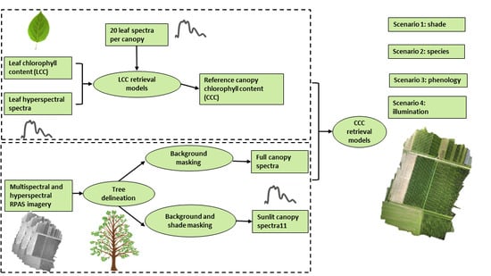
• shadow—we evaluate the CCC retrieval model shade sensitivity by comparing CCC retrieval models extracted from full and sunlit signals from both sensors;
• species—we evaluate the leaf chlorophyll content (LCC) and CCC retrieval model sensitivity of apple and pear species and both species combined from multi- and hyperspectral sensor systems;
• phenology—we evaluate the CCC retrieval model sensitivity to phenological stages by comparing the unitemporal with the multitemporal model performance;
• illumination differences—we evaluate the CCC retrieval model sensitivity to illumination differences by comparing the performance of unitemporal and multitemporal models on image acquisition days with cloudy and clear skies.

2. Materials and Methods

2.1. Study Area

Data for this study was collected during the growing season of 2017 from a pear (Pyrus communis) and apple (Malus Domestica) orchard in Belgium (Figure 1). The pear orchard, which was part of a drought and nitrogen treatment experiment, was located at the research station pcfruit (Proefcentrum Fruitteelt) in Kerkom, Belgium. The experimental design was composed of two adjacent rows with ‘Conference’ pear trees planted in 2000 on a Quince A rootstock with ‘Beurré Hardy’ and ‘Triomphe de Vienne’ as pollinators. Each row of 90 trees was divided in plots of five trees, consisting of three central experimental trees and two buffer trees. Three treatments were applied on the field: no nitrogen fertilization, double nitrogen fertilization (400 kg/ha Ca(NO₃)₂), and drought (induced by covering the soil with sails). There were also control plots which received standard nitrogen fertilization (200 kg/ha Ca(NO₃)₂). From each treatment, nine trees were selected to be monitored with ground measurements, thus 36 trees were selected in total.

The apple orchard, in which a fruitlet thinning experiment was conducted with metamitron, a chemical thinner, was located in Nieuwerkerken, Belgium. The experimental design, containing four adjacent rows with ‘Golden Delicious’ apple trees was planted in 2009. M9 was used as a rootstock and ‘Granny Smith’ as a pollinator. Each row was divided in plots of six trees, consisting of four central experimental trees and two buffer trees. Seven treatments were applied, differing in metamitron application timing with a dose rate of 247.5 g/ha. Each plot was treated with metamitron on another date, namely 16, 18, 22, 24, 26, and 30 May, and 1 June. These dates correspond to trees in the phenology BBCH (Biologische Bundesanstalt, Bundessortenamt und CHemische Industrie) stages of 69 (end of flowering (16–18 May)), 71 (fruit size up to 10 mm, fruit fall after flowering (22 May)) and 73 (second fruit fall (24 May–1 June) [34]. There were also control plots which received no thinning of the fruitlets. From each treatment and the control, all trees, so 48 in total, were monitored with ground measurements. A randomized block design was used to set-up both experiments. In this way, it was assumed that each plot in the field was influenced by similar environmental factors (e.g., soil type, moisture, weather). These experiments were expected to cause a wide range of chlorophyll values and were therefore chosen. The general characteristics and experimental design are provided in

Table A1. General characteristics and experimental design of the pear and apple orchard.

General Characteristics	Pear Orchard	Apple Orchard
Cultivar	Conference	Golden Delicious
Experiment	Drought-nutrient	Chemical thinning with metamitron
Rootstock	Quince C	M9
Planting year	2004	2009
Training system	Bush Spindle	Bush Spindle
Number of rows	2 rows	4 rows
Treatments	No nitrogen. Double nitrogen. Drought	7 different application times with metamitron
Total number of plots	16 plots	32 plots
Experimental trees per plot	6	3
Total number of trees in the experiment	76	96
Total number of monitored trees	36	48
Row distance × tree distance (m)	3.75 × 1.75	3 × 1.5
Mean tree height (m)	4.18	3

in the Appendix.

2.2. Remotely Piloted Aircraft System Imagery

Throughout the growing season of 2017 RPAS flights were conducted over the experimental orchards in May, June, July, August, and October. These dates correspond to different key moments in the growing season: the spring flush in May, the physiological and induced fruit drop in June, the vegetative growth stop, fruit growth and fruit ripening in July, harvest in August and September, and senescence in October [34]. Detailed information on the multispectral and hyperspectral flight campaign is summarized in

Table A2. Summary of the multispectral RPAS flight dates. date of the field spectrometer (ASD) measurements and growth stages.

Experimental Field	RPAS Multispectral	Acquisition Time RPAS Multispectral	Solar Noon	ASD	Growth Stage
Apple	17 May	01:24-01:36 p.m.	01:38 p.m.	23–25 May	Fruit fall after flowering (fruit size up to 10 mm) (BBCH71)
	14 June	09:07-09.21 a.m.	01:42 p.m.	12–19 June	Fruit size up to 20 mm, second fruit fall (BBCH 72-73)
	26 July	10:54-11:07 a.m.	01:49 p.m.	26–27 July	Fruit growth and ripening BBCH (73-87)
	29 August	03:00-03:14 p.m.	01:49 p.m.	4–7 September	Fruit ripe for picking (BBCH 87)
	16 October	08:30-08:43 a.m.	01:28 p.m.	12–13 October	Leaf senescence
Pear	17 May	03:32-03:50 p.m.	01:38 p.m.	30–31 May	Fruit fall after flowering, second fruit fall (BBCH 71-73)
	14 June	02:43-03:03 p.m.	01:42 p.m.	20–23 June	Second fruit fall (BBCH 72-73)
	13 July	11:47 a.m. - 12:12 p.m.	01:48 p.m.	18–19 July	Fruit growth and ripening (BBCH 73-87)
	22 August	10:17-10:33 a.m.	01:45 p.m.	14–16 August	Fruit ripe for picking (BBCH 87)
	16 October	12:54-01:09 p.m.	01:28 p.m.	12–13 October	Leaf senescence

and

Table A3. Summary of the hyperspectral RPAS flight dates. date of the field spectrometer (ASD) measurements and growth stages.

Experimental Field	RPAS Hyperspectral	Acquisition Time RPAS Hyperspectral	Solar Noon	ASD	Growth Stage
Apple	17 May	02:01-02:07 p.m.	01:38 p.m.	23–25 May	Fruit fall after flowering (fruit size up to 10 mm) (BBCH 71)
	14 June	12:08-12:15 p.m.	01:42 p.m.	12–19 June	Fruit size up to 20 mm, second fruit fall(BBCH 72-73)
			01:49 p.m.	26–27 July	Fruit growth and ripening BBCH (73-87)
	29 August	06:23-06:32 p.m.	01:43 p.m.	4–7 September	Fruit ripe for picking (BBCH 87)
Pear	17 May	03:58 – 04:06 p.m.	01:38 p.m.	30–31 May	Fruit fall after flowering, second fruit fall (BBCH 71-73)
	14 June	01:17-01:26 p.m.	01:42 p.m.	20–23 June	Second fruit fall (BBCH 72-73)
	13 July	02:20-02:27 p.m.	01:48 p.m.	18–19 July	Fruit growth and ripening (BBCH 73-87)
	22 August	11:24-11:32 a.m.	01:45 p.m.	14–16 August	Fruit ripe for picking (BBCH 87)
	16 October	03:29-03:35 p.m.	01:28 p.m.	12–13 October	Leaf senescence

in the Appendix. A detailed description of the sensor characteristics and preprocessing is given in the Supplementary Data. All datasets will be made available as part of BELAIR HESBANIA 2017 (SR/67/331a) [35].

2.2.1. Multispectral Imagery

The multispectral sensor Parrot Sequoia (Parrot Drone SAS, Paris, France) is a synchronized array of four single-band cameras (each with a similar 1.2 MP sensor with 3.75 µm pixel pitch and a 4 mm lens, but with a different interference filter in front of each sensor). These four bands are situated in the green (530–570 nm), red (640–680 nm), red-edge (730–740 nm), and near-infrared (770–810 nm) regions. The Parrot Sequoia was mounted inside the fixed-wing SenseFly eBee (SenseFly, Cheseaux-Losanne, Switserland) remotely piloted aircraft system. The spatial resolution of the multispectral images was 8 cm for a nominal flight height of 85 m above ground level, and images were acquired with 85% front- and sideward overlap. Images were processed through a structure from motion (SfM) photogrammetry workflow in the commercial software Agisoft PhotoScan 1.4.4. Before and after each flight, three four-band images were acquired from the calibration panel on the ground. In Agisoft PhotoScan, a reflectance calibration region of interest (ROI) was manually digitized on each band of the panel images, excluding edges and dirt spots. Then, the digital number (DN)-to-reflectance calibration was executed and transferred to all images, taking irradiance sensor values into account. Geometric correction is based on the use of ground control points in Agisoft PhotoScan. The alignment was run based on initial values of pixel pitch, focal length, and radial distortion, without self-calibrating parameters during the alignment (adaptive camera model fitting disabled). Then, the position of the real time kinematic (RTK) ground measurement on the marker was digitized on at least nine images for every marker visible in the flight imagery. Next, the camera self-calibration was run.

2.2.2. Hyperspectral Imagery

The hyperspectral Headwall Micro-Hyperspec sensor (Headwall Inc., USA), measures 326 bands in a spectral range of 400–1000 nm. The images have a spatial resolution of 5 cm at a normal flying height of 54 m. The sensor was mounted on the Altura Zenith ATX8 rotorcraft (Aerialtronics, The Netherlands). Simultaneously with the airborne data acquisition, ground reference data was collected from Ground Control Points (GCP’s) and a spectral reference target. This data was used for geometric and radiometric image calibration. For the radiometric and spectral calibration, the reference target, being a tarp with a reflectivity level of 36%, was manually selected from the hypercube. From this target area an average DN spectrum was created. Each spectrum from the hypercube was divided by this average DN spectrum and multiplied by the actual reflectance spectrum of the reflectance target. The latter was measured by the supplier of the target and is slightly wavelength dependent. Finally, a spline fit was performed on each hypercube spectrum using noise dependent smoothing factors to generate a smoothed reflectance hypercube. The geometric correction was performed using VITO’s own developed C++ module and was based on direct georeferencing. Input data from the sensor’s (Global Navigation Satellite Systems/Inertial Measurement Unit) GNSS/IMU, the sensor geometric model, boresight correction data and elevation data are further used during the geometric correction process. The data were projected to Lambert72 with an output pixel size of 5 × 5 cm.

2.3. Leaf Spectral Measurements

During the 2017 growing season, subsequent apple and pear leaf spectral measurements were taken as close as possible to the timing of each RPAS flight. Hyperspectral leaf measurements were collected using a Fieldspec 4 spectroradiometer (Malvern Panalytical, Longmont, CO, USA), with a contact probe and an attached light source. The internal stabilized light provided an even and reliable illumination source at selectable levels, ensuring consistent and properly directed full-range energy to the reference disk and samples. The radiometer measured in the range of 350–2500 nm. The sampling interval was 1.4 nm at 350–1050 nm, while it was 2 nm at the 1050–2500 nm spectral range. Before measuring the leaves, the ASD was optimized and a white reference was taken on spectralon. From each tree of the 36 pear and 48 apple trees, 10 top-shoot leaves and 10 middle-branch leaves were randomly selected, representing the canopy. Top-shoot leaves are assumed to make up a smaller part of the whole canopy but are closer to the nadir-looking sensor, while middle-shoot leaves contribute more to the whole canopy but overlap more with other branches and are at a larger distance from the sensor. Furthermore, a set of additional leaves was collected for which both the spectral reflectance was measured, and leaf chlorophyll destructively determined via chemical analysis (Section 2.6). The dataset comprised 204 pear (mean LCC = 55.5 μg/cm², range LCC = 0.7–91.9 μg/cm², standard deviation = 14.4 μg/cm²) and 183 apple leaves (mean LCC = 53.2 μg/cm², range LCC = 22–89.1 μg/cm², standard deviation = 13.2 μg/cm²) which were sampled throughout the growing season.

2.4. Phenology

The phenological growth stages for the apple and pear trees as specified through the BBCH code [34] are summarized in Table A2 and Table A3. Perennial pome fruit have a very rapid leaf area development in spring due to the existing structure, nutrient and carbon reserves. By bloom, the canopy of a mature tree has developed 20% of its maximal leaf area [36]. Full bloom was on 5 April for pear and two weeks later, on 18 April for apple. Apple physiological and induced fruit fall of small fruits occurred between 23 May and 19 June, while this was later for pear trees namely between 30 May and 23 June. Canopy development generally continues until midsummer [36]. Apple trees were picked mid-September, while the pear trees were already picked at the end of August. In mid-October, the timing of the last image acquisitions, leaf senescence and abscission had already started.

2.5. Chlorophyll Retrieval Workflow

Our workflow to retrieve canopy chlorophyll content from airborne multispectral and hyperspectral RPAS data comprised four steps (Figure 2). First, a species-independent leaf chlorophyll model was developed and applied to the leaf spectra, taken from each tree (Section 2.6). This gave us the reference CCC per individual tree. Second, individual canopies were detected, delineated, and masked for either background or background and shade from the RPAS imagery (Section 2.7). Third, the spectral information of each tree segment was extracted from the RPAS imagery to estimate the CCC with CCC retrieval models (Section 2.8). Fourth, the CCC retrieval model sensitivity was assessed under different scenarios of confounding factors (Section 2.9).

2.6. Reference Canopy Chlorophyll Content

The reference CCC, which is the real or ground reference chlorophyll content of each tree, was determined by averaging the LCC of 20 sampled leaves per tree (see Section 2.3). In order to establish a relation between the leaf spectral measurements taken by the ASD spectroradiometer and leaf chlorophyll content, a spectral calibration curve was built with the set of leaves which was collected throughout the growing season. After the leaf reflectance was measured according to the protocol described in Section 2.3, leaves were stored in an ice chest and transported to the lab. For chemical analysis, acetone was used as solvent to bring chlorophyll into solution. Absorbance was measured with a spectrophotometer at three wavelengths: 662, 645, and 740 nm [37]. Leaf chlorophyll content was determined by using these absorbances in the Lichenthaler and Buschmann (2001) [37] equations.

2.7. Tree Delineation and Masking

First, tree tops were identified on the canopy height model (CHM) of both the multispectral and hyperspectral imagery with an algorithm, searching for the maximum height in a window. Some tree tops needed to be manually adjusted by looking at tree shadow patterns on the grass. Each canopy top was then delineated using a circle with a diameter comprising the central part of the tree while preventing overlap with neighboring trees. Random forest classification was used to perform segmentation on the multispectral and hyperspectral data [38,39]. Training data comprised 10 polygons for the classes soil, sunlit sail, grass, shaded grass, sunlit canopy, and shaded canopy. Individual random forest models were developed for each image since the large illumination differences between imagery would demand an extensive training dataset to make a general model with a high accuracy feasible which was beyond the scope of this study. Accuracy metrics (overall accuracy > 0.9, Kappa > 0.9) of the random forest classification are given in the Supplementary Data. Background, defined as soil, sail, and shaded grass was masked in the multispectral image to retrieve the full canopy spectra. By averaging the spectra of all pixels belonging to one canopy, the full canopy spectrum was extracted (Figure A1). The class ‘sunlit grass’ could not be masked since it had too much overlap with the sunlit canopy class. For the hyperspectral imagery sunlit grass could be separated more easily from the sunlit canopy and therefore this class was also masked. For the sunlit canopy spectrum, only the sunlit pixels were averaged by also masking the canopy shade class (Figure A1).

2.8. Retrieval Models

Datasets for calibrating and validating LCC and CCC retrieval models were formed by combining the respective LCC with the leaf spectra and the combination of the reference CCC (Section 2.6) with the respective canopy spectrum (Section 2.7) of each tree for each month. Univariate and multivariate retrieval models were tested.

2.8.1. Univariate Retrieval Models

For the univariate models, three established chlorophyll and greenness indices were selected from relevant literature (

Table 1. Chlorophyll and greenness indices.

VI	Formula	Reference
NDVI	$\frac{\left(R_{\lambda 1}-R_{\lambda 2}\right)}{\left(R_{\lambda 1}+R_{\lambda 2}\right)}$	Rouse et al. (1974) [41]
TCARI	$3[\left(R_{700}-R_{670}\right)-0.2\left(R_{700}-R_{550}\right)\frac{R_{700}}{R_{670}}$	Haboudane et al. (2002) [42]
PRI	$\frac{R_{531}-R_{570}}{R_{531}+R_{570}}$	Gamon et al. (1992) [43]
REIP	700 + 40 *$\frac{\frac{R_{670}+R_{780}}{2}-R_{700}}{R_{740}+R_{700}}$	Guyot et al. (1988) [44]

) [22]. As the objective of this study was not to give an extensive overview of all existing chlorophyll vegetation indices, also a generic normalized difference vegetation index (NDVI) [40] was calculated, defined as NDVI with wavelengths λ1 and λ2 in order to provide the best correlation with the parameter of interest. This two-band index is optimized for local applications, but has shown to lack generic capacity in other studies [26].

2.8.2. Multivariate Retrieval Models

In this study, 15 multivariate models were selected based on reviews [26,45] and preliminary testing. This includes six linear models and 10 non-linear models. These models can further be divided in parametric and non-parametric methods. Additional information about these classes can be found in Moser et al. (2018) and James et al. (2013) [45,46]. Data processing and analyses were performed in the R statistical environment using the caret package [47] and the packages it is dependent upon (see

Table 2. Summary of the multivariate models.

Model Class	Model Subclass	Regression Model	Abbreviation	Package	Reference
Linear		Stepwise linear regression with sequential selection	RSS	leaps	[48]
Linear		Least angle regression	LARS	lars	[49]
Linear		Ridge regression	RR	elasticnet	[50]
Linear		Ridge regression with variable selection	RRVS	foba	[51]
Linear		Linear regression with elastic net	ENET	elasticnet	[50]
Linear		Projection pursuit regression	PPR	MASS	[52]
Non-linear	Decision tree	Random forest	RF	randomForest	[39]
Non-linear	Decision tree	Evolutionary algorithm for regression trees	TMGA	evtree	[53]
Non-linear	Decision tree	Stochastic gradient boosting	SGB	gbm	[54]
Non-linear	Kernel	Support vector machines with linear kernel	SVML	kernlab	[55]
Non-linear	Kernel	Support vector machines with radial kernel	SVMR	kernlab	[55]
Non-linear	Kernel	Gaussian processes regression with linear kernel	GPRL	kernlab	[55]
Non-linear	Kernel	Gaussian processes regression with radial kernel	GPRR	kernlab	[55]
Non-linear	Instance based and clustering	K-nearest neighbor	KNN	kknn	[56]
Non-linear	Instance based and clustering	Subtractive clustering and fuzzy c-means rules	SBC	frbs	[57]

).

Linear Models

The linear parametric models are all based on the standard linear regression model with p variables and with response y predicted by Equation (1). A model fitting procedure is applied to produce the vector of coefficients $\widehat{\beta }=({\widehat{\beta }}_0,\dots ,{\widehat{\beta }}_p)$. In stepwise linear regression with sequential selection (RSS) multiple regression is recursively applied a number of times. The process is a combination of forward and backward selection, evaluating a small number of subsets of variables by either adding or deleting variables one at a time [58]. The least angle regression (LARS) is also a linear regression model but is a computationally more efficient variant to the standard forward selection method. The LARS procedure works similar to linear regression with forward selection, starting with all coefficients equal to zero, and finding the variable most correlated with the response. Unlike standard forward selection, LARS proceeds in a direction equiangular between the two variables until a third variable is selected. LARS then proceeds equiangularly between these three variables, thus along the “least angle direction,” until a fourth variable enters and the process is repeated [59].

$$\widehat{y}={\widehat{\beta }}_0+x_1{\widehat{\beta }}_1+\dots +x_p{\widehat{\beta }}_p,$$

(1)

$$Y=X\beta +\epsilon ,$$

(2)

$$\widehat{\beta }={\left(x^{\prime }x\right)}^{-1}\left(x^{\prime }y\right).$$

(3)

In ridge regression (RR), the $\beta$ estimation procedure is based on adding small positive quantities to the diagonal of X’X (see Equation (3)). This adjustment is needed when the variables are multicollinear, which can be the case for hyperspectral data, leading to incorrect estimations of $\beta$ [60]. In ridge regression with variable selection (RRVS), variables are selected based on adaptive forward and backward selection [61]. Linear regression with elastic net (ENET) is also a combination of regularization and variable selection methods but based on LARS. This model encourages a grou** effect, where strongly correlated variables tend to be in or out of the model together. The elastic net is particularly useful when the number of variables largely exceeds the number of observations as is often the case with hyperspectral data [62]. Finally, a non-parametric linear regression technique, projection pursuit regression (PPR) was also explored. This method forms a linear combination of nonlinear functions [63].

Non-Linear Models

Non-linear multivariate retrieval models also referred to as machine learning regression algorithms apply non-linear transformations, assuming non-explicit relationships between variables [46]. These retrieval models are in this study divided in three large classes, namely (i) decision tree and additive models, (ii) kernel methods, and (iii) instance based or clustering models (Table 2). Based on the high potential of decision tree and additive models, three additional models were tested. First, an evolutionary algorithm for regression trees was applied. This algorithm first initializes a set of trees with random split rules in the root nodes. Second, mutation and crossover operators are applied to modify the trees’ structure and the tests that are applied in the internal nodes. After each modification step a survivor selection mechanism selects the best candidate models for the next iteration. In this evolutionary process the mean quality of the population increases over time [53]. Next, random forest (RF) was tested which gives as output the average prediction over a set of trained decision trees [38]. Finally, gradient boosting (SGB) was tested, which constructs additive regression models by sequentially fitting a simple parameterized function (weak learner) to current residuals by least-squares at each iteration. Specifically, at each iteration a subsample of the training data is drawn at random from the full training dataset. This randomly selected subsample is then used in place of the full sample to fit the weak learner and compute the model update for the current iteration. This randomized approach also increases robustness against overcapacity of the weak learner [64].

Kernel machines quantify similarities between input variables of a dataset. Similarity reproduces a linear dot product computed in a possibly higher dimensional feature space, yet without ever computing the data location in the feature space [26]. Support vector machines (SVMs) are a well-known example of kernel machines. SVMs integrate kernels with learning criteria that optimize generalization capability [65]. A support vector machine constructs a hyperplane or a set of hyperplanes in a high or even infinite dimensional space. Intuitively, one expects a good separation by application of a hyperplane, with the largest distance to the nearest training data point of any class [26]. Gaussian process regression is also a kernel technique but has a Bayesian distribution to describe relationships among the input variables. It is described by its mean and covariance as well. This represents an expected covariance between function values at a given point [26,65].

Instance-based models typically build up a database of example data and compare new data to the database using a similarity measure in order to find the best match and make a prediction. The nearest neighbor method (KNN) is such an instance-based model, both simple and nonparametric method, where a new observation is placed into the class of the observation from the learning set that is closest to the new observation, with respect to the covariates used [66]. Subtractive clustering and fuzzy c-means rules (SBC) uses a subtractive clustering method to obtain cluster centers. SBC considers each data point as a potential cluster center. A data point has a high potential value if that data point has many nearby neighbors. The highest potential is chosen as the cluster center. The process of determining new clusters and updating potentials repeats until the remaining potential of all data points falls below some fraction of the potential of the first cluster center. After getting all the cluster centers from subtractive clustering, the cluster centers are optimized by fuzzy c-mean [67].

2.9. Confounding Factors

In order to test the sensitivity of LCC and CCC retrieval models to confounding factors, main confounding factors were determined and evaluated in four different scenarios (canopy shade, species, phenology, and illumination) in the pome orchard scenery (Figure 2). Canopy shade differences within an orchard, result from tree size, variations in heights within canopies, and tree spacing [68]. Furthermore, shade fraction within the canopy is influenced by time of flight (sun angle). In order to prevent excessive shading, solar noon flights are recommended and applied in most studies. However, flying within a strict flight window limits potential coverage and revisit time of RPAS monitoring. By quantifying shade influence on the retrieval model accuracy, we can therefore decide if flying within this strict flight window is needed. CCC retrieval model sensitivity to shade was investigated by comparing the performance of retrieval models based on full and sunlit spectra of both multispectral and hyperspectral imagery. The influence of leaf parameters (i.e., biochemistry, specific leaf area, etc.) and canopy parameters (e.g., LAI, LAD, etc.) of apple and pear species was investigated by comparing the performance of individual species LCC and CCC retrieval models (i.e., apple and pear separately) with mixed species LCC and CCC retrieval models.

The best performing LCC model was applied on the LCC dataset collected in 2017 and the resulting LCC dynamics will be interpreted based on phenology and physiology. The species effect on the CCC retrieval models will be evaluated for both the multispectral and hyperspectral imagery. Since the influence of shade was already investigated in a previous section only sunlit spectra were included in this analysis. As previously mentioned in Section 2.3, apple and pear trees develop at a different pace, reaching phenological stages at different moments in time (Table A2 and Table A3). Therefore, CCC retrieval model sensitivity for specific dates (unitemporal) could be influenced by phenology. However, retrieval model performance can also be influenced by illumination differences due to clouds during image acquisition. CCC retrieval model sensitivity to phenological variations was tested for each species to gain insight in how well the multitemporal retrieval models perform on individual phenological stages, corresponding to individual months (i.e., unitemporal data) (Table A2 and Table A3). In addition, to assess the necessity of phenological stage specific models, the performance of unitemporal models was explored. These assessments were done for both sunlit multispectral and hyperspectral canopy spectra.

In order to quantify the effect of illumination variability, the performance of multi- and unitemporal CC retrieval models of a homogenously (i.e., clear sky or haze) and heterogeneously (i.e., cloudy) illuminated image were compared. For this objective, the July and August images were chosen since in July it was cloudy during the image acquisition for both orchards, while in August we had clear sky conditions during both flights. These two consecutive months were also chosen because the canopy is fully developed and the phenological stages are very close to each other. This entails that the model performance differences could largely be attributed to the differences in cloud cover.

2.10. Accuracy Assessment

The LCC and CCC datasets were partitioned in 80% training and 20% testing data, hence a five-fold cross-validation, which was repeated 10 times. This sampling distribution was found to be optimal in Verrelst et al. (2012b) [29]. The motivation being, that it is important to strive for accurate retrievals over a wide range of chlorophyll concentrations, requiring a wide range of training samples in the generation of the model. In turn, sufficient testing samples should be kept aside to employ a solid validation [29]. Chlorophyll retrieval model performance was tested with the accuracy metrics, coefficient of determination R² (Equation (4)), RMSE (Equation (5)) and Relative RMSE (RRMSE) (Equation (6)). The Root Mean Square Error (RMSE) was calculated to quantify the difference between the real and estimated chlorophyll content for all models. RMSE is a measure of the residual standard deviation and the closer to zero the better the fit. The RRMSE is the RMSE divided by the range of real chlorophyll content values.

$${\mathrm{R}}^2=\frac{{{\displaystyle \sum }}_{p=1}^k{\left({\mathrm{CC}}_{\mathrm{p}}^{*}-\overline{\mathrm{CC}}\right)}^2}{{{\displaystyle \sum }}_{p=1}^k{\left({\mathrm{CC}}_{\mathrm{p}}-\overline{\mathrm{CC}}\right)}^2},$$

(4)

$$\mathrm{RMSE}=\sqrt{{\displaystyle \sum }_{\mathrm{p}=1}^{\mathrm{k}}\frac{{\left({\mathrm{CC}}_{\mathrm{p}}^{*}-\overline{\mathrm{CC}}\right)}^2}{\mathrm{k}}}.$$

(5)

$$\mathrm{RRMSE}=\frac{\sqrt{{{\displaystyle \sum }}_{\mathrm{p}=1}^{\mathrm{k}}\frac{{\left({\mathrm{CC}}_{\mathrm{p}}^{*}-\overline{\mathrm{CC}}\right)}^2}{\mathrm{k}}}}{\mathrm{Max}\left({\mathrm{CC}}_{\mathrm{p}}\right)-\mathrm{Min}\left({\mathrm{CC}}_{\mathrm{p}}\right)}.$$

(6)

In Equations (4), (5), and (6) CCp is the reference chlorophyll content on leaf or canopy level, CCp* is the estimated chlorophyll content on leaf or canopy level, $\overline{\mathrm{CC}}$ is the average chlorophyll content on leaf or canopy level and k represents the number of measurements. For the LCC, k is equal to 204 for pear and 183 for apple. For the CCC, k is 48 for apple and 33 for pear for each month. In combination with Table A2 and Table A3 this attributes k equal to 144 (165) and 192 (165) CCC values for, respectively, the hyperspectral and multispectral imagery of apple (pear).

3. Results

3.1. Canopy Shade

We observed that the most accurate multivariate method outperformed the best performing vegetation indices by more than 12% and 15% respectively for the multispectral and hyperspectral data (Figure 3 and

Table A4. Mean R² (standard deviation), RMSE (standard deviation), and RRMSE statistics for the multispectral and hyperspectral data for retrieval of canopy chlorophyll content using the full and sunlit canopy spectrum.

Models	Multispectral Full Canopy Spectrum			Multispectral Sunlit Canopy Spectrum			Hyperspectral Full Canopy Spectrum			Hyperspectral Sunlit Canopy Spectrum
VI models	R2	RMSE	RRMSE	R2	RMSE	RRMSE	R2	RMSE	RRMSE	R2	RMSE	RRMSE
Best NDVI	0.50 (0.05)	4.83 (0.29)	20.0%	0.51 (0.05)	4.8 (0.30)	19.9%	0.53	4.41	18.3%	0.56	4.28	17.7%
TCARI/OSAVI	0.43 (0.07)	5.18 (0.36)	21.5%	0.49 (0.07)	4.9 (0.36)	20.3%	0.02 (0.02)	6.31 (0.17)	26.2%	0.03 (0.03)	5.63 (0.18)	23.3%
PRI	0.36 (0.07)	5.29 (0.32)	21.9%	0.51 (0.06)	4.8 (0.32)	19.9%	0.13 (0.06)	5.91 (0.25)	24.5%	0.13 (0.06)	5.23 (0.23)	21.7%
REIP	0.41 (0.08)	5.48 (0.38)	22.7%	0.59 (0.05)	4.4 (0.31)	18.2%	0.24 (0.07)	5.52 (0.28)	22.9%	0.22 (0.06)	4.78 (0.25)	19.8%
Linear multivariate models
RSS	0.58 (0.11)	4.43 (0.52)	18.4%	0.64 (0.05)	4.11 (0.31)	17.0%	0.63 (0.08)	3.86 (0.42)	16.0%	0.63 (0.08)	3.89 (0.45)	16.1%
LARS	0.58 (0.06)	4.44 (0.26)	18.4%	0.64 (0.06)	4.11 (0.28)	17.0%	0.76 (0.06)	3.08 (0.34)	12.8%	0.79 (0.06)	2.91 (0.30)	12.1%
ENET	0.58 (0.06)	4.43 (0.25)	18.4%	0.64 (0.06)	4.11 (0.27)	17.0%	0.70 9.00 (0.05)	2.91 (0.38)	12.1%	0.80 (0.06)	2.83 (0.40)	11.7%
RR	0.58 (0.05)	4.43 (0.28)	18.4%	0.64 (0.05)	4.12 (0.29)	17.1%	0.79 (0.05)	2.91 (0.39)	12.1%	0.80 (0.04)	2.83 (0.42)	11.7%
RRVS	0.58 (0.05)	4.43 (0.27)	18.4%	0.64 (0.05)	4.12 (0.31)	17.1%	0.78 (0.07)	3.03 (0.33)	12.6%	0.79 (0.08)	2.93 (0.45)	12.1%
PPR	0.66 (0.07)	4.00 (0.46)	16.6%	0.73 (0.07)	3.57 (0.48)	14.8%	0.59 (0.12)	4.44 (0.96)	18.4%	0.58 (0.15)	4.48 (1.15)	18.6%
Non-linear multivariate models
RF	0.70 (0.08)	3.84 (0.51)	15.9%	0.67 (0.09)	3.93 (0.52)	16.3%	0.72 (0.08)	3.40 (0.50)	14.1%	0.74 (0.07)	3.24 (0.48)	13.4%
TMGA	0.47 (0.09)	5.07 (0.43)	21.0%	0.54 (0.10)	4.71 (0.56)	19.5%	0.63 (0.11)	3.89 (0.63)	16.1%	0.65 (0.11)	3.78 (0.64)	15.7%
SGB	0.68 (0.07)	3.89 (0.38)	16.1%	0.67 (0.08)	3.91 (0.44)	16.2%	0.68 (0.09)	3.57 (0.50)	14.8%	0.73 (0.07)	3.29 (0.40)	13.6%
SVMR	0.77 (0.06)	3.3 (0.40)	13.7%	0.72 (0.07)	3.64 (0.41)	15.1%	0.74 (0.06)	3.21 (0.37)	13.3%	0.79 (0.04)	2.95 (0.29)	12.2%
SVML	0.58 (0.05)	4.46 (0.29)	18.5%	0.64 (0.05)	4.14 (0.31)	17.2%	0.73 (0.05)	3.28 (0.32)	13.6%	0.77 (0.04)	3.33 (0.29)	13.8%
GPRR	0.76 (0.05)	3.43 (0.37)	14.2%	0.72 (0.06)	3.67 (0.39)	15.2%	0.74 (0.05)	3.28 (0.31)	13.6%	0.78 (0.04)	3.05 (0.28)	12.6%
GPRL	0.58 (0.05)	4.45 (0.29)	18.4%	0.64 (0.05)	4.14 (0.31)	17.2%	0.73 (0.05)	3.30 (0.31)	13.7%	0.73 (0.06)	3.31 (0.36)	13.7%
KNN	0.78 (0.08)	3.22 (0.58)	13.3%	0.72 (0.08)	3.63 (0.56)	15.0%	0.77 (0.07)	3.02 (0.45)	12.5%	0.79 (0.05)	2.88 (0.37)	11.9%
SBC	0.53 (0.08)	4.75 (0.37)	19.7%	0.6 (0.08)	4.38 (0.37)	18.2%	0.75 (0.08)	3.19 (0.53)	13.2%	0.75 (0.07)	3.19 (0.47)	13.2%

). In general, multispectral indices had a higher accuracy than hyperspectral indices except for the NDVI. Sensor differences and the radiometric calibration as mentioned in Section 2.2 and the Supplementary Data both influence the signal to noise ratio of the images. For most multivariate models, lower RMSE’s and higher R² were achieved for the hyperspectral data (0.7 < R² < 0.8, RMSE < 3) than for the multispectral data (0.5 < R² < 0.7, RMSE < 4). Shade removal led to better retrieval accuracies for most methods. This effect was larger for the multispectral data (R² increased with 0.03 and RMSE decreased with 0.15) than for the hyperspectral data (R² increased with 0.02 and RMSE decreased with 0.10). Multivariate non-linear models and more specifically the kernel methods (0.73 < R² < 0.8) and RF (R² > 0.7) performed well for both the multispectral and hyperspectral imagery. These models also showed the highest robustness to shade. Using the full canopy in some cases even led to higher accuracies than limiting the spectrum to the sunlit pixels. While sunlit pixels are theorized to present tree status better, full canopy use leads to a bigger sample size. Multivariate linear models achieved high accuracies for the hyperspectral data (R² > 0.8) but were less suitable for the multispectral data (R² > 0.6). As noted in earlier research, linear models demand more features than non-linear models to fit non-linear relationships for achieving high accuracies [14,69].

3.2. Species Sensitivity

3.2.1. Leaf Chlorophyll Content

For both apple and pear, RSS provided the highest R² (0.88 for pear leaves, 0.82 for apple leaves) and lowest RMSE (5 µg/cm² for pear, 5.6 µg/cm² for apple) for LCC retrieval (

Table 3. Mean R² (standard deviation), Root Mean Square Error (RMSE) (standard deviation) and relative RMSE (RRMSE) statistics of the LCC retrieval models from hyperspectral data.

Models	Hyperspectral Leaf Spectrum			Hyperspectral Leaf Spectrum			Hyperspectral Leaf Spectrum
Species	Apple			Pear			Pear and Apple
VI models	R2	RMSE	RRMSE	R2	RMSE	RRMSE	R2	RMSE	RRMSE
Best NDVI	0.83 (0.05)	5.53 (0.56)	8.2%	0.87 (0.05)	5.17 (0.68)	5.7%	0.84 (0.03)	5.60 (0.45)	6.17%
TCARI/OSAVI	0.70 (0.06)	7.25 (0.72)	10.8%	0.61 (0.13)	9.35 (2.12)	10.3%	0.50 (0.07)	9.88 (0.92)	10.89%
PRI	0.30 (0.09)	11.00 (0.97)	16.4%	0.53 (0.16)	9.71 (0.82)	10.6%	0.43 (0.11)	10.46 (0.78)	11.53%
REIP	0.78 (0.06)	6.22 (0.65)	9.3%	0.61 (0.13)	12.00 (2.69)	13.2%	0.53 (0.13)	11.63 (3.67)	12.82%
Linear multivariate models
RSS	0.82 (0.07)	5.60 (0.99)	8.3%	0.88 (0.05)	5.01 (1.10)	5.5%	0.85 (0.05)	5.34 (0.78)	5.9%
LARS	0.79 (0.11)	6.05 (1.64)	9.0%	0.82 (0.14)	5.18 (3.66)	5.7%	0.85 (0.06)	5.42 (1.46)	5.9%
ENET	0.81 (0.09)	5.80 (1.34)	8.6%	0.87 (0.09)	5.24 (2.08)	5.7%	0.84 (0.06)	5.44 (1.04)	6.0%
RR	0.80 (0.10)	5.99 (1.51)	8.9%	0.87 (0.10)	5.52 (2.81)	6.1%	0.83 (0.06)	5.58 (1.31)	6.1%
RRVS	0.81 (0.08)	5.75 (1.11)	8.6%	0.88 (0.05)	5.02 (1.24)	5.5%	0.84 (0.06)	5.46 (1.02)	6.0%
PPR	0.51 (0.14)	11.17 (1.83)	16.7%	0.67 (0.23)	8.91 (3.60)	9.8%	0.77 (0.06)	6.89 (0.06)	7.6%
Non-Linear multivariate models
RF	0.77 (0.10)	6.30 (1.32)	9.4%	0.83 (0.10)	5.94 (1.89)	6.5%	0.78 (0.11)	6.40 (1.14)	7.0%
TMGA	0.67 (0.11)	7.77 (1.40)	11.6%	0.78 (0.13)	6.67 (1.52)	7.3%	0.69 (0.14)	7.59 (1.32)	8.3%
SGB	0.78 (0.07)	6.18 (1.01)	9.2%	0.79 (0.07)	6.90 (1.01)	7.6%	0.78 (0.08)	6.54 (0.97)	7.2%
SVMR	0.77 (0.09)	6.66 (1.34)	9.9%	0.69 (0.12)	7.28 (3.07)	8.0%	0.77 (0.09)	6.96 (1.77)	7.6%
SVML	0.80 (0.08)	5.82 (1.08)	8.7%	0.87 (0.05)	5.22 (1.26)	5.7%	0.77 (0.05)	5.48 (0.85)	6.0%
GPRR	0.70 (0.10)	7.54 (1.23)	11.2%	0.66 (0.11)	9.48 (2.77)	10.4%	0.67 (0.11)	8.47 (1.91)	9.3%
GPRL	0.80 (0.08)	5.87 (1.06)	8.8%	0.87 (0.05)	5.11 (1.04)	5.6%	0.84 (0.05)	5.45 (0.80)	6.0%
KNN	0.61 (0.15)	8.29 (1.49)	12.4%	0.74 (0.17)	7.56 (2.08)	8.3%	0.64 (0.11)	8.28 (1.03)	9.1%
SBC	0.53 (0.5)	9.33 (1.68)	13.9%	0.40 (0.19)	11.10 (1.87)	12.2%	0.51 (0.14)	9.64 (1.32)	10.6%

). RSS also had the highest accuracy for the mixed-species model (R² = 0.85, RMSE = 5.34 µg/cm²). However, taking into account the standard deviation of these metrics the difference in performance of the best vegetation index and the best performing multivariate method was negligible. As expected, the vegetation indices estimated the LCC with quite high accuracies. The coefficient of determination is similar to the multitemporal LCC retrieval models accuracy for apple R² = 0.83 [70] and R² = 0.85 for pear [15] in other research. Apple and pear leaf chlorophyll dynamics retrieved from the LCC retrieval model are shown in Figure 4. LCC ranged from 40 to 50 µg/cm² in May and stayed relatively stable until June for apple while showing a small increase for pear. Between June and July LCC increased for apple, reaching 57–65 µg/cm². For pear this increase was slower, reaching its peak in August with values ranging from 55 to 65 µg/cm². At the end of August, beginning of September, LCC began decreasing with the onset of senescence to 40–50 µg/cm² for pear and 47–55 µg/cm² for apple.

3.2.2. Canopy Chlorophyll Content

The multivariate methods again outperformed the vegetation indices, but this observation was less pronounced for the apple trees than for the pear trees (Figure 5). The hyperspectral apple specific models (apple: RSS, RRVS, RF, SGB: R² = 0.90–0.91, RRMSE = 9%) (

Table A5. Mean R² (standard deviation), RMSE (standard deviation), and RRMSE statistics of the CCC retrieval models from sunlit hyperspectral RPAS imagery.

Models	Hyperspectral Sunlit Canopy Spectrum			Hyperspectral Sunlit Canopy Spectrum			Hyperspectral Sunlit Canopy Spectrum
Species	Apple			Pear			Pear and Apple
VI models	R2	RMSE	RRMSE	R2	RMSE	RRMSE	R2	RMSE	RRMSE
Best NDVI	0.83	2.79	12.6%	0.36	4.67	19.4%	0.56	4.28	17.7%
TCARI/OSAVI	0.25 (0.14)	5.80 (0.60)	26.2%	0.06 (0.13)	5.76 (0.48)	23.9%	0.03 (0.03)	5.63 (0.18)	23.3%
PRI	0.43 (0.16)	5.09 (0.75)	23.0%	0.18 (0.10)	5.30 (0.33)	22.0%	0.13 (0.06)	5.23 (0.23)	21.7%
REIP	0.55 (0.08)	4.48 (0.42)	20.3%	0.30 (0.12)	4.94 (0.43)	20.5%	0.22 (0.06)	4.78 (0.25)	19.8%
Linear multivariate models
RSS	0.91 (0.02)	2.03 (0.23)	9.2%	0.61 (0.12)	4.69 (0.67)	19.4%	0.63 (0.05)	3.89 (0.45)	16.1%
LARS	0.91 (0.05)	2.24 (0.54)	10.1%	0.73 (0.08)	3.22 (0.35)	13.3%	0.79 (0.06)	2.91 (0.64)	12.1%
ENET	0.90 (0.05)	2.10 (0.63)	9.5%	0.82 (0.15)	2.49 (0.53)	10.3%	0.80 (0.06)	2.83 (0.40)	11.7%
RR	0.91 (0.04)	2.13 (0.12)	9.6%	0.82 (0.13)	2.49 (0.55)	10.3%	0.80 (0.04)	2.83 (0.42)	11.7%
RRVS	0.91 (0.04)	2.03 (0.42)	9.2%	0.82 (0.10)	2.54 (0.42)	10.5%	0.79 (0.08)	2.93 (0.45)	12.1%
PRR	0.41 (0.17)	6.39 (0.13)	28.9%	0.70 (0.09)	3.44 (0.54)	14.3%	0.58 (0.15)	4.48 (1.15)	18.6%
Non-linear multivariate models
RF	0.90 (0.02)	2.09 (0.22)	9.4%	0.60 (0.12)	3.66 (0.54)	15.2%	0.74 (0.07)	3.24 (0.48)	13.4%
TMGA	0.87 (0.09)	2.28 (0.72)	10.3%	0.47 (0.14)	4.24 (0.64)	17.6%	0.65 (0.11)	3.78 (0.64)	15.7%
SGB	0.91 (0.02)	2.04 (0.22)	9.2%	0.54 (0.12)	3.91 (0.53)	16.2%	0.73 (0.07)	3.29 (0.40)	13.6%
SVMR	0.90 (0.03)	2.16 (0.22)	9.8%	0.57 (0.09)	3.82 (0.43)	15.8%	0.79 (0.04)	2.95 (0.29)	12.2%
SVML	0.90 (0.02)	2.09 (0.26)	9.4%	0.78 (0.07)	2.75 (0.39)	11.4%	0.77 (0.04)	3.33 (0.29)	13.8%
GPRR	0.87 (0.03)	2.53 (0.30)	11.4%	0.58 (0.09)	3.92 (0.43)	16.2%	0.78 (0.04)	3.05 (0.28)	12.6%
GPRL	0.91 (0.02)	2.05 (0.22)	9.3%	0.77 (0.12)	2.81 (0.55)	11.6%	0.73 (0.06)	3.31 (0.36)	13.7%
KNN	0.91 (0.02)	2.05 (0.20)	9.3%	0.62 (0.12)	3.59 (0.55)	14.9%	0.79 (0.05)	2.88 (0.37)	11.9%
SBC	0.87 (0.03)	2.53 (0.03)	11.4%	0.60 (0.14)	3.70 (0.71)	15.3%	0.75 (0.07)	3.19 (0.47)	13.2%

) outperformed the multispectral apple specific models (apple: PPR: R² = 0.77, RRMSE = 15%) (

Table A6. Mean R² (standard deviation), RMSE (standard deviation), and RRMSE statistics of the CCC retrieval models from sunlit multispectral RPAS imagery.

Models	Multispectral Sunlit Canopy Spectrum			Multispectral Sunlit Canopy Spectrum			Multispectral Sunlit Canopy Spectrum
Species	Apple			Pear			Pear and Apple
VI models	R2	RMSE	RRMSE	R2	RMSE	RRMSE	R2	RMSE	RRMSE
Best NDVI	0.72 (0.06)	4.12 (0.41)	17.2%	0.62 (0.07)	3.58 (0.35)	14.8%	0.51 (0.05)	4.80 (0.30)	19.9%
TCARI/OSAVI	0.74 (0.09)	3.96 (0.48)	16.5%	0.43 (0.09)	4.32 (0.41)	17.9%	0.49 (0.07)	4.90 (0.36)	20.3%
PRI	0.72 (0.08)	4.12 (0.41)	17.2%	0.38 (0.03)	4.55 (0.33)	18.9%	0.51 (0.06)	4.80 (0.32)	19.9%
REIP	0.66 (0.05)	4.54 (0.38)	18.9%	0.62 (0.09)	3.56 (0.38)	14.8%	0.59 (0.05)	4.40 (0.31)	18.2%
Linear multivariate models
RSS	0.69 (0.07)	4.33 (0.46)	18.1%	0.66 (0.11)	3.40 (0.49)	14.1%	0.64 (0.05)	4.11 (0.31)	17.0%
LARS	0.69 (0.07)	4.33 (0.37)	18.1%	0.66 (0.09)	3.39 (0.34)	14.0%	0.64 (0.06)	4.11 (0.28)	17.0%
ENET	0.69 (0.06)	4.33 (0.34)	18.1%	0.66 (0.10)	3.39 (0.38)	14.0%	0.64 (0.06)	4.11 (0.27)	17.0%
RR	0.69 (0.06)	4.33 (0.39)	18.1%	0.66 (0.09)	3.39 (0.44)	14.0%	0.64 (0.05)	4.12 (0.29)	17.1%
RRVS	0.69 (0.06)	4.33 (0.40)	18.1%	0.66 (0.09)	3.39 (0.42)	14.0%	0.64 (0.05)	4.12 (0.31)	17.1%
PPR	0.77 (0.07)	3.67 (0.62)	15.3%	0.70 (0.09)	3.16 (0.50)	13.1%	0.73 (0.07)	3.57 (0.48)	14.8%
Non-linear multivariate models
RF	0.68 (0.09)	4.32 (0.59)	18.0%	0.77 (0.08)	2.78 (0.54)	11.5%	0.67 (0.09)	3.93 (0.52)	16.3%
TMGA	0.60 (0.13)	4.97 (0.83)	20.7%	0.63 (0.15)	3.60 (0.75)	14.9%	0.54 (0.10)	4.71 (0.56)	19.5%
SGB	0.68 (0.08)	4.35 (0.51)	18.1%	0.71 (0.09)	3.10 (0.53)	12.8%	0.67 (0.08)	3.91 (0.44)	16.2%
SVMR	0.70 (0.07)	4.24 (0.47)	17.7%	0.80 (0.05)	2.63 (0.33)	10.9%	0.72 (0.07)	3.64 (0.41)	15.1%
SVML	0.68 (0.05)	4.38 (0.38)	18.3%	0.65 (0.08)	2.63 (0.44)	10.9%	0.64 (0.05)	4.14 (0.31)	17.2%
GPRR	0.70 (0.06)	4.32 (0.43)	18.0%	0.81 (0.05)	2.66 (0.31)	11.0%	0.72 (0.06)	3.67 (0.39)	15.2%
GPRL	0.68 (0.05)	4.35 (0.37)	18.1%	0.65 (0.08)	3.43 (0.42)	14.2%	0.64 (0.05)	4.14 (0.31)	17.2%
KNN	0.67 (0.09)	4.45 (0.60)	18.6%	0.84 (0.05)	2.35 (0.35)	9.7%	0.72 (0.08)	3.63 (0.56)	15.0%
SBC	0.59 (0.09)	5.00 (0.48)	20.9%	0.79 (0.08)	2.66 (0.42)	11.0%	0.60 (0.08)	4.38 (0.37)	18.2%

). It is striking that the linear methods, thus both vegetation indices and the linear multivariate models, gave the highest accuracies for the apple trees. For pear, the difference between the best performing hyperspectral and multispectral models was smaller (pear hyperspectral: ENET, RR, RRVS: R² = 0.82, RRMSE = 10%; pear multispectral: KNN R² = 0.84, RRMSE = 10%). In general, the hyperspectral pear models performed worse than the hyperspectral apple models, while they performed more similarly for the multispectral data.

The lower performance of the hyperspectral pear models compared to the multispectral pear models (Figure 5) was unexpected. Therefore, the relationship between the canopy spectra of the multispectral and hyperspectral sensor was investigated for each month separately and all months together (

Table 4. R² between the multispectral and resampled hyperspectral canopy spectra.

	Band	All	May	June	July	August	October
Pear	Green	<0.01	0.34	0.59	0.54	0.07	0.67
	Red	0.06	0.25	0.55	0.23	0.09	0.78
	Red edge	0.03	0.21	0.27	0.57	<0.01	0.26
	NIR	0.03	0.27	0.3	0.6	<0.01	0.4
Apple	Green	0.13	0.03	0.02	/	0.19	/
	Red	0.01	0.1	0.09	/	0.19	/
	Red edge	0.35	0.21	0.05	/	0.08	/
	NIR	0.27	0.27	<0.01	/	0.1	/

). The hyperspectral canopy spectra were resampled to the spectral resolution of the multispectral sensor assuming a gaussian distribution. For all months, except for August, the correlation between the multispectral and resampled hyperspectral canopy pear spectra was very poor to high (0.2 < R² < 0.7). The August spectra of pear and the apple spectra of all months had a very poor to medium correlation (0.01 < R² < 0.35). The low correlations for those months was likely due to the difference in flight plan between the multispectral and hyperspectral imagery, leading to a different canopy-sensor-sun geometry (see Supplementary Data). For the months with medium to high correlation, the hyperspectral sensor was flown parallel to the orientation of the fruit tree rows, while for the other months the hyperspectral sensor was flown perpendicular to the row orientation. In addition, there was a difference in solar position for the different sensors (Table A2 and Table A3) and a difference in projection of the trees due to the lower overlap of the hyperspectral sensor compared to the multispectral sensor (see Supplementary Data).

In

Table A7. Mean R² (standard deviation), RMSE (standard deviation), and RRMSE statistics of the CCC retrieval models from hyperspectral RPAS imagery (without pear August).

	Hyperspectral Sunlit			Hyperspectral Sunlit			Hyperspectral Sunlit
Models	Apple			Pear			Pear and Apple
VI models	R2	RMSE	RRMSE	R2	RMSE	RRMSE	R2	RMSE	RRMSE
Best NDVI	0.83	2.79	12.6%	0.54	2.98	15.3%	0.54	3.84	17.3%
TCARI/OSAVI	0.25 (0.14)	5.80 (0.60)	26.2%	0.08 (0.12)	4.23 (0.41)	21.7%	0.05 (0.03)	5.54 (0.25)	25.0%
PRI	0.43 (0.16)	5.09 (0.75)	23.0%	0.09 (0.08)	4.13 (0.30)	21.2%	0.11 (0.06)	5.33 (0.25)	24.0%
REIP	0.55 (0.08)	4.48 (0.42)	20.3%	0.13 (0.09)	4.05 (0.30)	20.8%	0.18 (0.09)	5.13 (0.32)	23.1%
Linear multivariate models
RSS	0.91 (0.02)	2.03 (0.23)	9.2%	0.60 (0.11)	2.78 (0.48)	15.9%	0.73 (0.08)	3.64 (0.33)	16.4%
LARS	0.91 (0.05)	2.24 (0.54)	10.1%	0.61 (0.09)	2.97 (0.41)	16.8%	0.80 (0.06)	2.82 (0.26)	12.7%
ENET	0.90 (0.05)	2.10 (0.63)	9.5%	0.70 (0.11)	2.46 (0.65)	13.8%	0.80 (0.05)	2.76 (0.25)	12.4%
RR	0.91 (0.04)	2.13 (0.12)	9.6%	0.69 (0.11)	2.49 (0.82)	13.9%	0.80 (0.04)	2.82 (0.23)	12.7%
RRVS	0.91 (0.04)	2.03 (0.42)	9.2%	0.70 (0.10)	2.43 (0.43)	13.9%	0.78 (0.06)	3.07 (0.27)	13.8%
PPR	0.41 (0.17)	6.39 (0.13)	28.9%	0.49 (0.15)	3.78 (0.72)	21.8%	0.67 (0.13)	4.45 (0.83)	20.1%
Non-linear multivariate models
RF	0.90 (0.02)	2.09 (0.22)	9.4%	0.52 (0.12)	3.04 (0.42)	16.7%	0.80 (0.06)	2.92 (0.33)	13.2%
TMGA	0.87 (0.09)	2.28 (0.72)	10.3%	0.38 (0.11)	3.51 (0.44)	19.7%	0.76 (0.08)	3.32 (0.39)	15.0%
SGB	0.91 (0.02)	2.04 (0.22)	9.2%	0.51 (0.12)	3.01 (0.42)	16.1%	0.80 (0.07)	2.82 (0.31)	12.7%
SVMR	0.90 (0.03)	2.16 (0.22)	9.8%	0.53 (0.12)	2.97 (0.35)	16.5%	0.81 (0.05)	2.79 (0.29)	12.6%
SVML	0.90 (0.02)	2.09 (0.26)	9.4%	0.71 (0.08)	2.40 (0.41)	13.5%	0.77 (0.06)	3.07 (0.29)	13.8%
GPRR	0.87 (0.03)	2.53 (0.30)	11.4%	0.53 (0.12)	3.06 (0.34)	17.0%	0.81 (0.04)	2.79 (0.26)	12.6%
GPRL	0.91 (0.02)	2.05 (0.22)	9.3%	0.70 (0.08)	2.43 (0.42)	13.9%	0.77 (0.03)	3.05 (0.24)	13.7%
KNN	0.91 (0.02)	2.05 (0.20)	9.3%	0.51 (0.10)	3.15 (0.35)	16.7%	0.82 (0.04)	2.63 (0.21)	11.9%
SBC	0.87 (0.03)	2.53 (0.03)	11.4%	0.48 (0.12)	3.28 (0.48)	18.3%	0.78 (0.05)	3.03 (0.28)	13.7%

, the results of the CCC retrieval from the sunlit hyperspectral imagery is given, excluding the hyperspectral imagery of pear for August. This led to a decrease in accuracy for the individual hyperspectral pear CCC models but an increase of the accuracy of the mixed species hyperspectral CCC models. Excluding August decreased the range of chlorophyll values (Figure 4) leading to lower R² for pear but the mixed models were still based on the high chlorophyll values of apple to compensate for this loss.

3.3. Unitemporal versus Multitemporal

3.3.1. Unitemporal

Results of the univariate and multivariate unitemporal CCC retrieval models of apple and pear can be found in

Table A8. R² accuracy metric of unitemporal CCC retrieval models for pear (apple) trees from sunlit multispectral data.

	Weather	ENET	LARS	RSS	PPR	RR	RRVS	SBC	GPRL	GPRR	KNN	RF	SVML	SVMR	TMGA	BestVI
May		0.21 (0.14)	0.21 (0.14)	0.22 (0.13)	0.23 (0.17)	0.24 (0.12)	0.30 (0.26)	0.26 (0.07)	0.24 (0.12)	0.20 (0.06)	0.22 (0.09)	0.26 (0.08)	0.25 (0.12)	0.15 (0.06)	0.24 (0.10)	0.23 (0.67)
June		0.20 (0.11)	0.20 (0.11)	0.24 (0.13)	0.17 (0.12)	0.21 (0.13)	0.25 (0.08)	0.22 (0.10)	0.20 (0.14)	0.21 (0.07)	0.24 (0.07)	0.16 (0.11)	0.19 (0.15)	0.13 (0.07)	0.28 (0.13)	0.21 (0.12)
July		0.14 (0.11)	0.14 (0.09)	0.14 (0.09)	0.19 (0.10)	0.15 (0.10)	0.21 (0.10)	0.16 (0.08)	0.15 (0.10)	0.15 (0.09)	0.15 (0.07)	0.21 (0.14)	0.18 (0.11)	0.16 (0.08)	0.09 (0.08)	0.25 (0.13)
August		0.19 (0.10)	0.19 (0.08)	0.17 (0.09)	0.16 (0.07)	0.14 (0.08)	0.09 (0.14)	0.17 (0.08)	0.15 (0.08)	0.20 (0.09)	0.20 (0.24)	0.15 (0.19)	0.11 (0.10)	0.23 (0.10)	0.19 (0.23)	0.24 (0.11)
October		0.26	0.26	0.29	0.21	0.27	0.31	0.15	0.26	0.12	0.20	0.16	0.27	0.12	0.14	0.37

and

Table A9. R² accuracy metric of unitemporal CCC retrieval models for pear (apple) trees from sunlit hyperspectral data.

	Weather	ENET	LARS	RSS	PPR	RR	RRVS	SBC	GPRL	GPRR	KNN	RF	SVML	SVMR	TMGA
May		0.20 (0.10)	0.16 (0.08)	0.18 (0.10)	0.18 (0.14)	0.19 (0.10)	0.21 (0.11)	0.19 (0.08)	0.18 (0.10)	0.20 (0.19)	0.21 (0.07)	0.15 (0.19)	0.15 (0.08)	0.21 (0.19)	0.19 (0.07)
June		0.16 (0.10)	0.14 (0.13)	0.15 (0.11)	0.17 (0.23)	0.14 (0.12)	0.20 (0.08)	0.19 (0.11)	0.15 (0.12)	0.11 (0.15)	0.25 (0.16)	0.13 (0.07)	0.17 (0.11)	0.13 (0.12)	0.23 (0.15)
July		0.24	0.19	0.24	0.18	0.21	0.32	0.20	0.21	0.20	0.18	0.15	0.20	0.23	0.11
August		0.25 (0.10)	0.19 (0.08)	0.19 (0.16)	0.18 (0.19)	0.19 (0.09)	0.22 (0.10)	0.13 (0.12)	0.18 (0.09)	0.10 (0.14)	0.20 (0.10)	0.12 (0.08)	0.18 (0.09)	0.23 (0.14)	0.15 (0.14)
October		0.19	0.13	0.13	0.23	0.09	0.23	0.13	0.08	0.15	0.22	0.13	0.16	0.14	0.21

. In general, the unitemporal CCC retrieval models have a low performance with most R² < 0.30. This is the case for both multispectral and hyperspectral imagery. There is one outlier in May with a R² of 0.67 for apple for the multispectral data. The R² of unitemporal univariate models is more consistent over the growing season compared to that of multivariate models.

3.3.2. Multitemporal

Most of the multitemporal models have a very poor accuracy R² < 0.3 (

Table 5. R² accuracy metric of multitemporal CCC retrieval models for pear (apple) trees from sunlit multispectral data.

	Weather	ENET	LARS	RSS	PPR	RR	RRVS	SBC	GPRL	GPRR	KNN	RF	SVML	SVMR	TMGA	BestVI
May		0.00 (0.04)	0.00 (0.04)	0.00 (0.04)	0.01 (0.1)	0.00 (0.04)	0.00 (0.04)	0.10 (0.15)	0.00 (0.04)	0.26 (0.01)	0.07 (0.02)	0.45 (0.81)	0.00 (0.04)	0.60 (0.04)	0.01 (0.04)	0 (0.05)
June		0.01 (0)	0.01 (0)	0.01 (0)	0.01 (0.1)	0.01 (0)	0.01 (0)	0.04 (0)	0.01 (0)	0.14 (0.01)	0.15 (0.01)	0.82 (0.35)	0.01 (0)	0.47 (0.01)	0.02 (0.01)	0 (0)
July		0.02 (0)	0.02 (0)	0.02 (0)	0.00 (0.07)	0.0 (0.02)	0.02 (0)	0.07 (0.01)	0.03 (0)	0.21 (0.03)	0.01 (0.01)	0.71 (0.26)	0.03 (0)	0.29 (0.03)	0.08 (0)	0.04 (0)
August		0.04 (0.02)	0.04 (0.02)	0.04 (0.02)	0.01 (0.01)	0.04 (0.02)	0.04 (0.02)	0.16 (0.04)	0.03 (0.02)	0.15 (0)	0.12 (0.07)	0.70 (0.32)	0.03 (0.01)	0.35 (0.03)	0.00 (0.01)	0.01 (0.03)
October		0.13	0.13	0.13	0.00	0.13	0.14	0.01	0.17	0.20	0.02	0.72	0.11	0.24	0.00	0.24

,

Table 6. R² accuracy metric of multitemporal CCC retrieval models for all trees from sunlit multispectral data.

	Weather	ENET	LARS	RSS	PPR	RR	RRVS	SBC	GPRL	GPRR	KNN	RF	SVML	SVMR	TMGA	SGB
May		0.67	0.71	0.67	0.86	0.67	0.67	0.86	0.69	0.86	0.94	0.97	0.86	0.86	0.79	0.9
June		0.08	0.04	0.08	0.52	0.08	0.08	0.16	0.07	0.56	0.64	0.9	0.09	0.65	0.75	0.72
July		0.61	0.59	0.61	0.76	0.61	0.61	0.62	0.59	0.79	0.9	0.97	0.61	0.83	0.8	0.84
August		0.61	0.58	0.61	0.82	0.61	0.61	0.75	0.61	0.78	0.84	0.95	0.59	0.75	0.81	0.87
October		0.01	0.07	<0.01	<0.01	0.01	0.01	0.28	0.02	0.04	0.04	0.49	0.03	0.09	0.24	0.11

,

Table 7. R² accuracy metric of multitemporal CCC retrieval models for pear (apple) trees from hyperspectral data.

	Weather	ENET	LARS	RSS	PPR	RR	RRVS	SBC	GPRL	GPRR	KNN	RF	SVML	SVMR	TMGA
May		0.19 (0.31)	0.60 (0.72)	0.00 (0)	0.86 (0.99)	0.24 (0.05)	0.24 (0)	0.32 (0.88)	0.04 (0.47)	0.02 (0.30)	0.16 (0.27)	0.46 (0.92)	0.07 (0.5)	0.07 (0.5)	0.00 (0)
June		0.10 (0)	0.49 (0.39)	0.09 (0)	0.79 (0.39)	0.14 (0)	0.12 (0)	0.29 (0.98)	0.08 (0.01)	0.09 (0.20)	0.02 (0.18)	0.66 (0.9)	0.10 (0.04)	0.15 (0)	0.08 (0)
July		0.05	0.62	0.06	0.76	0.10	0.12	0.48	0.00	0.07	0.04	0.52	0.00	0.07	0.00
August		0.04 (0.15)	0.70 (0.76)	0.03 (0.04)	0.56 (0.99)	0.04 (0.12)	0.05 (0.05)	0.88 (0.99)	0.06 (0.32)	0.07 (0.06)	0.02 (0.09)	0.23 (0.91)	0.04 (0.38)	0.15 (0.4)	0.08 (0)
October		0.18	0.94	0.06	0.96	0.26	0.32	0.99	0.01	0.27	0.09	0.51	0.03	0.27	0.01

and

Table 8. R² accuracy metric of multitemporal CCC retrieval models for pear trees from hyperspectral data (without August).

	Weather	ENET	LARS	RSS	PPR	RR	RRVS	SBC	GPRL	GPRR	KNN	RF	SVML	SVMR	TMGA	SGB
May		0.24	0.56	0.09	0.79	0.31	0.03	0.85	0.17	0.04	0.06	0.45	0.22	0.14	0	0.79
June		0.08	0.55	<0.01	0.84	0.14	0.56	0.56	0.03	0.06	0.12	0.73	0.06	0.18	0.06	0.86
July		0.11	0.61	<0.01	0.76	0.16	0.03	0.61	0.03	0.15	0.34	0.61	0.02	0.07	0.01	0.66
October		0.29	0.92	<0.01	0.95	0.38	0.08	0.99	0.08	0.63	0.5	0.93	0.06	0.74	0.07	0.86

). Yet, some multitemporal models have medium to high accuracies (0.3 < R² < 0.99) for most individual months. For the multispectral imagery, the RF multitemporal model performs best for all months for apple and pear trees individually (Table 5) and mixed (Table 6). For May, the RF model for apples performs best, while for the other months the performance of the pear RF model is better. For mixed species, the CCC model on sunlit multispectral imagery (Table 6) PPR, SBC, GPRR, SVMR, GBM, and RF give high accuracies for all months, except for October. RF is the only model giving a mediocre accuracy for October (R² = 0.5) and very high accuracies for the other months (R² > 0.9). The mixed multitemporal RF model (Table 6) for the multispectral imagery also outperforms the individual species models (0.5 < R² < 0.97 versus 0.26 < R² < 0.82) (Table 5), except for October.

For the sunlit hyperspectral imagery (Table 7) two linear (LARS and PPR) and two non-linear (SBC and RF) multivariate models give the best results. PPR and RF give the most steady and highest performance for pear and apple trees respectively. For each individual month, CCC is retrieved with the highest accuracy with PPR on hyperspectral data for the pear trees, except for August (PPR May R² = 0.86, June R² = 0.79, July R² = 0.76, October R² = 0.96), where SBC leads to higher accuracies (SBC: R² = 0.88 versus PPR: R² = 0.56) (Table 7). For apple trees, both SBC and RF give very high accuracies for all months R² > 0.9 (Table 7), while PPR has a higher accuracy for May and August but has a low accuracy for June (R² < 0.4). LARS is the fastest multivariate regression model but had mediocre to high retrieval accuracies (0.4 < R² < 0.94) for the hyperspectral data of apple and pear (Table 7). In order to see the effect of row orientation on the retrieval accuracies (Section 3.2.1), the hyperspectral image of August was removed for the pear trees (Table 8). This increased the retrieval accuracies of RF for the months July and October by 17% and 82% compared to the model with August included. For SBC, the exclusion of August led to increased accuracies for May and June (165% and 93%) but a decrease in accuracy for July (31%). The other models were less affected by the exclusion of the August imagery. Sunlit hyperspectral CCC retrieval models for mixed species were also evaluated for each month separately (

Table A10. R² accuracy metric of multitemporal CCC retrieval models for all trees from hyperspectral data with August and (without August of pear).

	Weather	ENET	LARS	RSS	PPR	RR	RRVS	SBC	GPRL	GPRR	KNN	RF	SVML	SVMR	TMGA	SGB
May		0.28 (0.31)	0.26 (0.33)	0.09 (0.14)	0.59 (0.61)	0.28 (0.37)	0.35 (0.45)	0.49 (0.55)	0.16 (0.23)	0.29 (0.32)	0.5 (0.5)	0.73 (0.75)	0.16 (0.59)	0.37 (0.23)	0.18 (0.40)	0.65 (0.18)
June		0.6 (0.63)	0.57 (0.63)	0.39 (0.42)	0.76 (0.80)	0.60 (0.65)	0.63 (0.66)	0.83 (0.84)	0.47 (0.56)	0.74 (0.74)	0.85 (0.85)	0.9 (0.89)	0.47 (0.81)	0.79 (0.58)	0.68 (0.79)	0.82 (0.64)
July		0.03 (<0.01)	0.02 (<0.01)	<0.01 (<0.01)	0.38 (0.33)	0.03 (<0.01)	0.02 (<0.01)	0.3 (0.47)	<0.01 (<0.01)	0.03 (0.05)	0.31 (0.30)	0.57 (0.56)	<0.01 (0.32)	0.03 (0.02)	0.01 (0.04)	0.22 (0.02)
August		0.06 (0.03)	0.03 (0.03)	0.07 (0.02)	0.71 (0.54)	0.06 (0.06)	0.1 (0.13)	0.9 (0.96)	<0.01 (<0.01)	0.07 (0.07)	0.31 (0.59)	0.5 (0.68)	0.03 (0.36)	0.24 (<0.01)	<0.01 (0.26)	0.44 (<0.01)
October		0.02 (0.04)	<0.01 (0.05)	0.02 (<0.01)	0.61 (0.72)	0.02 (0.08)	0.07 (0.15)	0.99 (0.99)	0.01 (<0.01)	0.16 (0.41)	0.08 (0.57)	0.08 (0.85)	<0.01 (0.61)	0.18 (<0.01)	0.22 (0.46)	0.56 (0.11)

). RF, PPR, and SBC deliver consistently the highest accuracies (0.3 < R² < 0.99) for the hyperspectral imagery. From these models, RF is the most consistent of all the models, reaching similar accuracies for each month (0.6 < R² < 0.9), while the PPR and SBC reach very high accuracies for some months (June, August, and October) and medium to even low accuracies for other months (May and July). The removal of the August hyperspectral imagery of the pear orchard was important to reach these high accuracies for August.

4. Discussion

4.1. Physiological and Phenological Interpretation of CCC Dynamics

To our knowledge absolute numbers of CCC differences between fruit trees and over the full growing season have never been reported for a relatively large sample of fruit trees. In addition, we want to see if our results can be supported with the body of knowledge regarding fruit tree phenology and physiology. CCC differences between trees within one month provide insight into the physiological performance, while CCC differences from one month to the other offer information on tree phenology [71]. As leaves mature, chlorophyll accumulates in the leaves from May until July or August (Figure 4). The increase in CCC from June until July for Golden Delicious was also observed by Prsa et al. (2007) [4]. The sharpness of the peak in July was dependent on tree nitrogen status, the lower the nitrogen fertilization, the steeper the peak in July [4] and thus the steeper the fall of CCC in August.

From July (apple)/August (pear) onwards, chlorophyll was degraded during senescence unraveling carotenoids and anthocyanins [72]. From early September until November, a further constant loss of CCC in apple trees was in agreement with the findings of Spencer et al. (1973) [73]. Presence of fruit on the trees was observed to delay chlorophyll degradation [74]. However, this was not the case in this study since the pear trees were picked first on August 29, followed by the apple trees on September 12. This could be due to the fact that the effect of crop load on leaf senescence is species specific. However, the decrease in CCC was stronger for the pear than for apple from August to October. In both trials (Table A1), stressors (i.e., metamitron, nitrogen deficit, drought) were applied to cause within month CCC differences since these stressors influence photosynthetic activity, for which chlorophyll is a strong indicator (Figure 6 and Figure 7) [4,42,75]. However, the effect of the treatments on the chlorophyll content of the trees was smaller than expected with only a reduced chlorophyll content of trees stressed with drought compared to the other treatments (Figure 7).

4.2. Confounding Factor Identification, Importance, and Mitigation

The higher number of bands of the hyperspectral imagery (i.e., 280 bands) compared to the multispectral imagery (i.e., 4 bands) led to the higher general performance of these models for all confounding factors (Figure 3). However, multispectral indices had a higher accuracy than hyperspectral indices except for the NDVI. The former is in contrast to expectations since previous research showed that narrowband indices exceed wide band index accuracy [76]. Noise, which plays a larger role in narrow band indices is a likely source of this observation [77]. The presence of shade had no impact on the retrieval accuracies of the multitemporal multivariate multispectral (R² decrease of 0.03 and RMSE increase by 0.15) and hyperspectral CCC models (R² decrease of 0.02 and RMSE increase by 0.10). The high performing models can benefit from the entire wealth of available features (e.g., PPR, RR, SBC) while it offers other models the flexibility to select the best bands to mitigate the influence of confounding factors (e.g., ENET, LARS, RRVS, RF). Models belonging to the first class will need all bands available in the hyperspectral sensor, while models in the second class offer the opportunity to develop a custom-made commercial multispectral sensor by identifying the most informative bands. While the hyperspectral vegetation indices did not decrease in accuracy due to the presence of shade, the multispectral vegetation indices were strongly impacted by the presence of shade with a decrease in accuracy between R² = 0.01 and 0.18 (Table A4).

4.2.1. Tree Architecture, Shade, and Crop Load Differences between Species

Mixed and species-specific model performance were compared to test the potential of a generic model for pome fruit trees. LCC retrieval models performed generally better (Table 3) than the CCC retrieval models (Figure 5 and Table A7) due to the fact that there are fewer confounding factors since leaves are measured in a controlled environment. Multispectral species-specific models for apple and pear outperformed the mixed-species models (Figure 5). For the hyperspectral sensor, only the apple specific model led to higher accuracies compared to the mixed model (Figure 5). One of the main causes of the lower accuracy of the species specific pear CCC retrieval models was probably the August imagery (odels performed generally better (Table 4, Table 8 and Table A10). The August imagery of the pear orchard was different from the other months because of its deviating flight plan: the RPAS was flown perpendicular to the orchard rows, while it was flown parallel to the rows on other dates, leading to a different field of view of the trees hence adding an additional confounding factor in the imagery. Ideally, the RPAS platform was flown with sunlight parallel to the rows of the fruit orchard. This was not always feasible due to strict airspace regulations.

In addition, tree architecture might explain the differences in model robustness for both species. Although both tree species were trained in spindle, they did differ in their height-width ratio, overall canopy shape, and age. Pear tree classical training system is characterized by very sparse branches and leaves for most of the tree height, with leaves clustered mostly on a small lower tree region. In general, classical trained pear trees have a 50% smaller leaf cover area and larger leaf wall porosity than the apple classical training system for most of the tree height [12]. These characteristics of pear trees likely led to higher within canopy shading and more background presence, introducing additional noise and thus explaining the lower accuracy of the species-specific pear hyperspectral CCC retrieval models. Furthermore, the flight time influences the percentage of shade as well. In May and October, hyperspectral image acquisition for the pear orchard was outside the recommended flight window (Table A3). In May, the canopy was not yet fully developed (see Section 2.4) leading to an even more discontinuous canopy [78]. In addition, the weather was cloudy over the orchard during the May image acquisition.

However, in August there was also a hyperspectral image acquisition over the apple orchard outside the recommended flight window but as sunset was setting in (Table A3). A low sun elevation angle in combination with diffuse light reduces within canopy shading for this tree shape [79]. However, shade pixels proved to have a negligible negative impact on the retrieval accuracies for the hyperspectral and multispectral models in this study (Figure 3). While sunlit pixels are theorized to present tree status better, full canopy use leads to a bigger sample size. A low shade fraction in combination with a fully developed canopy in August (Section 2.4) had probably minor negative impacts on the retrieval accuracy for apple. In addition, in July and August, pear fruits already thickened more than apple fruit (Table A2), hence contributing to the canopy signal but the chlorophyll content of the fruits was not taken into account with the ground measurements. The presence of fruit decreases canopy reflectance in the near infrared regions of the canopy spectrum (700–900 nm) [21], while this region and specifically the red edge (point of maximum slope between VIS and NIR), proved to be very important for LCC and CCC retrieval [80,81,82]. Finally, the hyperspectral apple data was more homogenous than the hyperspectral pear data since both contained the same amount of sample data but spread over five months for the pear trees but only for three months for the apple data (Table A3). Hence the same amount of observations is used to handle a higher heterogeneity in confounding factors (i.e., field of view, phenology, tree architecture, shade fraction) for the pear trees.

4.2.2. Illumination Variability Caused by Weather

Illumination conditions, thus favorably a clear sky, could not be proven to be a determining factor for retrieval accuracies for all multitemporal models (e.g., August, October (clear sky) versus May, June, and July (haze and cloudy) (Table 5 and Table 6). Only for the hyperspectral LARS and SBC model an increase in R² can be seen for clear sky days (i.e., August. October) compared to days with haze (i.e., May, June) or cloudy days (i.e., July) (Table 7). Phenology and illumination conditions varied on most flight days (Table A2 and Table A3) so these confounding factors could not be uncoupled for most months except for July and August. For these consecutive months, tree phenology is assumed to be quite similar since the canopy stops develo** mid-summer (Section 2.4) but illumination conditions were different on both dates. Hence these months are ideal to uncouple the phenology effect and the illumination effect. Only the hyperspectral LARS, SBC (Table 7), and the multispectral RF (Table 6) showed higher R² accuracies for August compared to July. Therefore, even for the months with similar phenology, illumination conditions could not be proven to have a negative impact on all retrieval models.

4.3. Multispectral versus Hyperspectral CCC Monitoring in Practice

For monitoring the average seasonal CCC dynamics of both apple and pear trees the hyperspectral models (i.e., ENET, RR, RRVS, and KNN) give a slightly higher accuracy (R² = 0.8. RRMSE = 12%) compared to the best performing multispectral models (i.e., PPR, SVMR, GPRR, and KNN with R² = 0.72–0.73, RRMSE = 15%) (Table A4). However, from a practical point of view, retrieving the CCC variability between trees on one date with a high accuracy is more important. CCC variations within a single orchard were better monitored with multitemporal (Table 5, Table 6, Table 7 and Table 8) than with unitemporal models (Table A8 and Table A9). Possible causes for the low performance of unitemporal models were probably a combination of the large BRDF effects due to the complex tree architecture [30] in combination with the relatively small within orchard variability in CCC in the trials compared to the between month CCC variability (Figure 4, Figure 6 and Figure 7). In addition, a smaller sample size for model calibration was available for the unitemporal (33–48 samples) versus the multitemporal modelling (144–240 samples) to diminish the effect of the confounding factors over the parameter of interest. Low sample sizes lead to lower retrieval accuracies and a higher variability in retrieval models [83]. GPR models even demand over 600 samples to achieve optimal accuracies [84].

For estimating CCC differences between trees on a single month, the multitemporal RF model gave the most consistent and in general, highest retrieval accuracies on the multispectral imagery (R² > 0.9 for May, June, July, and August and R² = 0.5 for October) (Table 6) and hyperspectral imagery (0.6 < R² < 0.9 for all months) (Table A10). The higher performance of the hyperspectral compared to the multispectral CCC retrieval model for October (R² = 0.85 versus R² = 0.49) is likely due to an under sampling during the senescence period in October. During senescence, the chlorophyll content of the leaves decreases (Figure 4, Figure 6 and Figure 7), while anthocyanin content remains constant or increases, leading to a stronger interference with the spectral region important for chlorophyll retrieval [85]. The mixed model (Table 6) even outperformed the species specific models (Table 5) for the individual months of the multispectral imagery. This is in contrast with the earlier observations (Figure 5) where the species specific models always outperformed the mixed models. This is probably also caused by the sample size. In Figure 5 the sampling points of all months are combined, while in Table 5 the model performance is tested on sampling points of only one month. For the hyperspectral imagery, the apple species specific RF model (Table 7) still outperforms the mixed RF model (Table 8). The uniformity of the flight plan and tree architecture probably overruled the effect of the smaller sample size in this case.

Other models which performed similar but less consistent than RF, were PPR and SBC. PPR and SBC are not frequently used for remote sensing applications but in an extensive study on the performance of 77 regression models on 48 datasets, PPR ranked 13^th, RF ranked 6^th and SBC did not even make the top 20 of best performing models. For small but difficult datasets RF ranks even higher at position 3 and for small but easy datasets PPR ranks position 6. The fact that SBC was ranked so low could be due to long running time errors which occurred for 85% of the investigated datasets since the model is quite slow [86]. In addition, the regression rules family to which SBC belongs in ranks the first position. However, in contrast to SBC and PPR, RF does not need all available bands and reaches moderate accuracies (R²~0.7) with 10 bands and maximal accuracy with 40 bands. This offers the opportunity to generate a custom-made MS sensor. However, the commercial MS sensor in this study already gives satisfying results for most months with RF to retrieve the CCC with R² > 0.9.

4.4. Limitations and Recommendations for Future Research

This study was limited to CCC retrieval in fruit orchards, since our goal was to develop and evaluate a RPAS chlorophyll monitoring system for fruit orchards as an alternative to field measurements. Tree delineation and shade removal were very labor-intensive steps, not ready for full automatization and beyond the scope of this paper. A robust and automatized method to delineate fruit trees was however explored in recent research on citrus trees [87]. In this study, the best performing classes of models and specific models were identified. For the objectives of this study the models were kept in their default settings. However, some classes of multivariate models could be further improved by optimized band selection [69], hyper parameter optimization [88], or active learning to select the best observations to build the retrieval models [84]. Furthermore, data reduction methods were not explored but can also further improve the retrieval models. The importance of the lack of BRDF correction in RPAS preprocessing chains is known [30] but was not quantified in this study and hence only indirectly studied as part of the other confounding factors. It would be interesting to quantify the BRDF effects and correct for them [15,89]. This would reduce the noise and lead to higher retrieval accuracies for the multispectral sensor. Instead of removing the noise, different viewing geometries of the sensor could also be used to give a more complete image of the canopy, resulting in better retrieval accuracies for tree parameters since a larger sample of the canopy is taken into account [90]. Data collection to calibrate models was very labor-intensive, therefore the importance of stage specific phenology models could not be proven or refuted due to the limited sample set for each month. Moreover, data collection for this study was limited to two orchards in one year. The methodology should be transferrable to other orchards and years. However, additional training data might be needed to address the different confounding factors present in these orchards to reach the same accuracy levels. In this study we looked at the average spectrum per tree. It would also be interesting to use the high spatial resolution to spot chlorophyll content differences within the canopy [5] since these patterns can inform growers about the type of stress the tree is experiencing.

5. Conclusions

The main objective of this study was to develop a robust CCC retrieval model for pome fruit tree monitoring using RPAS platforms equipped with an optical sensor. Chlorophyll is an important variable for steering management practices. Yet, orchard scenery complexity prevented a comprehensive assessment of the full potential of this technology for operational use in earlier studies. In this paper the accuracies of 15 multivariate and four univariate models were compared in four scenarios: the presence of within canopy shade, species (i.e., apple, pear, and mixed), phenology, and illumination conditions (i.e., weather). In addition, the economically priced multispectral sensor Sequioa was also compared to the more expensive hyperspectral sensor Microhyperspec. Through the evaluation of chlorophyll retrieval models on multispectral and hyperspectral time series, the importance of confounding factors was highlighted, while it was demonstrated that multitemporal multivariate models outperformed all other retrieval models. Overall, the most important conclusions of the current study can be summarized as follows. Random Forest, Subtractive clustering and fuzzy c-means rules and Projection pursuit regression are the preferred multivariate models to most accurately monitor the chlorophyll dynamics for apple and pear trees. Random forest however outperforms the other models in consistency, robustness and needs less bands to reach a high accuracy. Both the multitemporal Random Forest on multispectral imagery (R² > 0.9 for May, June, July, and August and R² = 0.5 for October) and hyperspectral imagery (0.6 < R² < 0.9) led to satisfactory high retrieval accuracies. An advantage of the hyperspectral sensor was that there were more bands available to mitigate the effects of shade (i.e., vegetation indices), the interference of anthocyanins (i.e., October), and species (i.e., apple, pear). However, the availability of bands could not correct for the difference in field of view (FOV) on one date (i.e., August) and additional sample heterogeneity (i.e., pear versus apple). Finally, since the multispectral sensor is cheaper for practical use in the orchard during the growing season, it would be preferable to use the random forest model on the Sequoia multispectral imagery or a custom-made sensor. For the senescence period, more data should be collected to see if the model performance on the multispectral imagery can be improved or if hyperspectral imagery will need to be used.

References

1. Blackburn, A. Hyperspectral remote sensing of plant pigments. Comp. Biochem. Physiol. Mol. Integr. Physiol. 2006, 143, S147. [Google Scholar] [CrossRef] [PubMed]
2. Bolat, I.; Dikilitas, M.; Ercisli, S.; Ikinci, A.; Tonkaz, T. The effect of water stress on some morphological, physiological, and biochemical characteristics and bud success on apple and Quince rootstocks. Sci. World J. 2014. [Google Scholar] [CrossRef] [PubMed]
3. Amarante, C.V.T.d.; Steffens, C.A.; Mafra, Á.L.; Albuquerque, J.A. Yield and fruit quality of apple from conventional and organic production systems. Pesqui. Agropecu. Bras. 2008, 43, 333–340. [Google Scholar] [CrossRef]
4. Prsa, I.; Stampar, F.; Vodnik, D.; Veberic, R. Influence of nitrogen on leaf chlorophyll content and photosynthesis of ‘Golden Delicious’ apple. Acta Agric. Scand. Sect. B Soil Plant Sci. 2007, 57, 283–289. [Google Scholar] [CrossRef]
5. Ma, X.; Feng, J.; Guan, H.; Liu, G. Prediction of chlorophyll content in different light areas of apple tree canopies based on the color characteristics of 3D reconstruction. Remote Sens. 2018, 10, 429. [Google Scholar] [CrossRef]
6. Perry, E.M.; Davenport, J.R. Spectral and spatial differences in response of vegetation indices to nitrogen treatments on apple. Comput. Electron. Agric. 2007, 59, 56–65. [Google Scholar] [CrossRef]
7. Li, C.; Zhu, X.; Wei, Y.; Cao, S.; Guo, X.; Yu, X.; Chang, C. Estimating apple tree canopy chlorophyll content based on Sentinel-2A remote sensing imaging. Sci. Rep. 2018, 8, 3756. [Google Scholar] [CrossRef] [PubMed]
8. Somers, B.; Cools, K.; Delalieux, S.; Stuckens, J.; Van der Zande, D.; Verstraeten, W.W.; Coppin, P. Nonlinear hyperspectral mixture analysis for tree cover estimates in orchards. Remote Sens. Environ. 2009, 113, 1183–1193. [Google Scholar] [CrossRef]
9. Van Beek, J.; Tits, L.; Somers, B.; Coppin, P. Stem water potential monitoring in pear orchards through WorldView-2 multispectral imagery. Remote Sens. 2013, 5, 6647–6666. [Google Scholar] [CrossRef]
10. Thenkabail, P.S.; Lyon, J.G.; Huete, A. Advances in Hyperspectral Remote Sens. of Vegetation and Agricultural Croplands; CRC Press: Boca Raton, FL, USA, 2012. [Google Scholar]
11. Berni, J.A.J.; Zarco-Tejada, P.J.; Suarez, L.; Fereres, E. Thermal and Narrowband Multispectral Remote Sensing for Vegetation Monitoring from an Unmanned Aerial Vehicle. IEEE Trans. Geosci. Remote Sens. 2009, 47, 722–738. [Google Scholar] [CrossRef]
12. Duga, A.T.; Ruysen, K.; Dekeyser, D.; Nuyttens, D.; Bylemans, D.; Nicolai, B.M.; Verboven, P. Spray deposition profiles in pome fruit trees: Effects of sprayer design, training system and tree canopy characteristics. Crop Prot. 2015, 67, 200–213. [Google Scholar] [CrossRef]
13. Verrelst, J.; Alonso, L.; Camps-Valls, G.; Delegido, J.; Moreno, J. Retrieval of vegetation biophysical parameters using Gaussian process techniques. IEEE Trans. Geosci. Remote Sens. 2012, 50, 1832–1843. [Google Scholar] [CrossRef]
14. Degerickx, J.; Roberts, D.; McFadden, J.; Hermy, M.; Somers, B. Urban tree health assessment using airborne hyperspectral and LiDAR imagery. Int. J. Appl. Earth Obs. Geoinf. 2018, 73, 26–38. [Google Scholar] [CrossRef] [Green Version]
15. Van Beek, J.; Tits, L.; Somers, B.; Deckers, T.; Janssens, P.; Coppin, P. Viewing geometry sensitivity of commonly used vegetation indices towards the estimation of biophysical variables in orchards. J. Imaging 2016, 2, 15. [Google Scholar] [CrossRef]
16. **, J.; Wang, Q. Informative bands used by efficient hyperspectral indices to predict leaf biochemical contents are determined by their relative absorptions. Int. J. Appl. Earth Obs. Geoinf. 2018, 73, 616–626. [Google Scholar] [CrossRef]
17. Féret, J.-B.; Gitelson, A.; Noble, S.; Jacquemoud, S. PROSPECT-D: Towards modeling leaf optical properties through a complete lifecycle. Remote Sens. Environ. 2017, 193, 204–215. [Google Scholar] [CrossRef] [Green Version]
18. Cui, R.; Qin, Q.; Yang, N.; Tao, X.; Zhao, S. The optimization of the crop chlorophyll content indices based on a new LAI determination index. In Proceedings of the 2009 IEEE International Geoscience and Remote Sensing Symposium, Cape Town, South Africa, 12–17 July 2009; pp. IV-821–IV-824. [Google Scholar]
19. Zou, X.; Hernández-Clemente, R.; Tammeorg, P.; Lizarazo Torres, C.; Stoddard, F.L.; Mäkelä, P.; Pellikka, P.; Mõttus, M. Retrieval of leaf chlorophyll content in field crops using narrow-band indices: Effects of leaf area index and leaf mean tilt angle. Int. J. Remote Sens. 2015, 36, 6031–6055. [Google Scholar] [CrossRef]
20. Delalieux, S.; Somers, B.; Hereijgers, S.; Verstraeten, W.; Keulemans, W.; Coppin, P. A near-infrared narrow-waveband ratio to determine Leaf Area Index in orchards. Remote Sens. Environ. 2008, 112, 3762–3772. [Google Scholar] [CrossRef]
21. Somers, B.; Delalieux, S.; Verstraeten, W.W.; Eynde, A.V.; Barry, G.H.; Coppin, P. The contribution of the fruit component to the hyperspectral citrus canopy signal. Photogramm. Eng. Remote Sens. 2010, 76, 37–47. [Google Scholar] [CrossRef]
22. Aasen, H.; Bolten, A. Multi-temporal high-resolution imaging spectroscopy with hyperspectral 2D imagers—From theory to application. Remote Sens. Environ. 2018, 205, 374–389. [Google Scholar] [CrossRef]
23. Kunz, A.; Blanke, M. Effects of global climate change on apple ‘Golden Delicious’ phenology based on 50 years of meteorological and phenological data in Klein-Altendorf. In Proceedings of the IX International Symposium on Integrating Canopy, Rootstock and Environmental Physiology in Orchard Systems, Geneva, NY, USA, 4–8 August 2008; pp. 1121–1126. [Google Scholar]
24. Lakso, A.N. Apple. In Handbook of Environmental Physiology of Fruit Crops; CRC Press: Boca Raton, FL, USA, 1994; pp. 3–42. [Google Scholar]
25. Darbyshire, R.; Farrera, I.; Martinez-Lüscher, J.; Leite, G.B.; Mathieu, V.; El Yaacoubi, A.; Legave, J.-M. A global evaluation of apple flowering phenology models for climate adaptation. Agric. For. Meteorol. 2017, 240, 67–77. [Google Scholar] [CrossRef]
26. Verrelst, J.; Camps-Valls, G.; Munoz-Mari, J.; Rivera, J.P.; Veroustraete, F.; Clevers, J.; Moreno, J. Optical remote sensing and the retrieval of terrestrial vegetation bio-geophysical properties—A review. ISPRS J. Photogramm. Remote Sens. 2015, 108, 273–290. [Google Scholar] [CrossRef]
27. Stuckens, J.; Somers, B.; Delalieux, S.; Verstraeten, W.; Coppin, P. The impact of common assumptions on canopy radiative transfer simulations: A case study in Citrus orchards. J. Quant. Spectrosc. Radiat. Transf. 2009, 110, 1–21. [Google Scholar] [CrossRef]
28. Koetz, B.; Baret, F.; Poilvé, H.; Hill, J. Use of coupled canopy structure dynamic and radiative transfer models to estimate biophysical canopy characteristics. Remote Sens. Environ. 2005, 95, 115–124. [Google Scholar] [CrossRef]
29. Verrelst, J.; Munoz, J.; Alonso, L.; Delegido, J.; Rivera, J.P.; Camps-Valls, G.; Moreno, J. Machine learning regression algorithms for biophysical parameter retrieval: Opportunities for Sentinel-2 and -3. Remote Sens. Environ. 2012, 118, 127–139. [Google Scholar] [CrossRef]
30. Tu, Y.-H.; Phinn, S.; Johansen, K.; Robson, A. Assessing radiometric correction approaches for multi-spectral UAS imagery for horticultural applications. Remote Sens. 2018, 10, 1684. [Google Scholar] [CrossRef]
31. Suomalainen, J.; Anders, N.; Iqbal, S.; Roerink, G.; Franke, J.; Wenting, P.; Hünniger, D.; Bartholomeus, H.; Becker, R.; Kooistra, L. A lightweight hyperspectral map** system and photogrammetric processing chain for unmanned aerial vehicles. Remote Sens. 2014, 6, 11013–11030. [Google Scholar] [CrossRef]
32. Pádua, L.; Vanko, J.; Hruška, J.; Adão, T.; Sousa, J.J.; Peres, E.; Morais, R. UAS, sensors, and data processing in agroforestry: A review towards practical applications. Int. J. Remote Sens. 2017, 38, 2349–2391. [Google Scholar] [CrossRef]
33. Adão, T.; Hruška, J.; Pádua, L.; Bessa, J.; Peres, E.; Morais, R.; Sousa, J. Hyperspectral imaging: A review on UAV-based sensors, data processing and applications for agriculture and forestry. Remote Sens. 2017, 9, 1110. [Google Scholar] [CrossRef]
34. Meier, U.; Graf, H.; Hack, H.; Hess, M.; Kennel, W.; Klose, R.; Mappes, D.; Seipp, D.; Stauss, R.; Streif, J. Phanologische Entwicklungsstadien des Kernobstes (Malus domestica Borkh. und Pyrus communis L.), des Steinobstes (Prunus-Arten), der Johannisbeere Ribes-Arten) und der Erdbeere (Fragaria x ananassa. Nachrichtenblatt Dtsch. Pflanzenschutzd. 1994, 46, 141–153. [Google Scholar]
35. Belair Hesbania Dataset 2017; KULeuven, V. (Ed.) VITO: Mol, Belgium, 2019. [Google Scholar]
36. Lakso, A.; Wünsche, J.; Palmer, J.; Corelli Grappadelli, L. Measurement and modeling of carbon balance of the apple tree. HortScience 1999, 34, 1040–1047. [Google Scholar] [CrossRef]
37. Lichtenthaler, H.K.; Buschmann, C. Chlorophylls and carotenoids: Measurement and characterization by UV-VIS spectroscopy. Curr. Protoc. Food Anal. Chem. 2001, 1. [Google Scholar] [CrossRef]
38. Breiman, L. Random forests. Mach. Learn. 2001, 45, 5–32. [Google Scholar] [CrossRef]
39. Liaw, A.; Wiener, M. Classification and Regression by randomForest. R News 2002, 2, 18–22. [Google Scholar]
40. Delalieux, S.; Somers, B.; Verstraeten, W.; Van Aardt, J.; Keulemans, W.; Coppin, P. Hyperspectral indices to diagnose leaf biotic stress of apple plants, considering leaf phenology. Int. J. Remote Sens. 2009, 30, 1887–1912. [Google Scholar] [CrossRef]
41. Rouse, J., Jr.; Haas, R.; Deering, D.; Schell, J.; Harlan, J. Monitoring the Vernal Advancement and Retrogradation (Green Wave Effect) of Natural Vegetation. [Great Plains Corridor]; NASA: Washington, DC, USA, 1974.
42. Haboudane, D.; Miller, J.R.; Tremblay, N.; Zarco-Tejada, P.J.; Dextraze, L. Integrated narrow-band vegetation indices for prediction of crop chlorophyll content for application to precision agriculture. Remote Sens. Environ. 2002, 81, 416–426. [Google Scholar] [CrossRef]
43. Gamon, J.; Penuelas, J.; Field, C. A narrow-waveband spectral index that tracks diurnal changes in photosynthetic efficiency. Remote Sens. Environ. 1992, 41, 35–44. [Google Scholar] [CrossRef]
44. Guyot, G.; Baret, F.; Major, D. High spectral resolution: Determination of spectral shifts between the red and the near infrared. Int. Arch. Photogramm. Remote Sens. 1988, 11, 750–760. [Google Scholar]
45. Moser, G.; Zerubia, J.; Serpico, S.B.; Benediktsson, J.A. Mathematical Models and Methods for Remote Sensing Image Analysis: An Introduction. In Mathematical Models for Remote Sens. Image Processing: Models and Methods for the Analysis of 2D Satellite and Aerial Images; Moser, G., Zerubia, J., Eds.; Springer International Publishing: Cham, Switzerland, 2018; pp. 1–36. [Google Scholar]
46. James, G.; Witten, D.; Hastie, T.; Tibshirani, R. An Introduction to Statistical Learning; Springer: New York, NY, USA, 2013; Volume 2. [Google Scholar]
47. Kuhn, M. Building predictive models in R using the caret package. J. Stat. Softw. 2008, 28, 1–26. [Google Scholar] [CrossRef]
48. Lumley, T. Leaps: Regression Subset Selection; R Package Version 3, Fortran Code by Alan Miller; 2017. Available online: https://cran.r-project.org/ (accessed on 19 June 2019).
49. Hastie, T.; Efron, B. Lars: Least Angle Regression, Lasso and Forward Stagewise; R Package Version 1.2; 2013. Available online: https://cran.r-project.org/ (accessed on 19 June 2019).
50. Zou, H.; Hastie, T. Elasticnet: Elastic-Net for Sparse Estimation and Sparse PCA.; R Package Version 1.1; 2012. Available online: https://cran.r-project.org/ (accessed on 19 June 2019).
51. Zhang, T. Foba: Greedy Variable Selection; R package Version 0.1; 2008. Available online: https://cran.r-project.org/ (accessed on 19 June 2019).
52. Venables, W.N.; Ripley, B.D. Modern Applied Statistics with S, 4th ed.; Springer: New York, NY, USA, 2002. [Google Scholar]
53. Grubinger, T.; Zeileis, A.; Pfeiffer, K.-P. Evtree: Evolutionary Learning of Globally Optimal Classification and Regression Trees in R; Working Papers in Economics and Statistics; Universität Innsbruck: Innsbruck, Austria, 2011. [Google Scholar]
54. Ridgeway, G. Gbm: Generalized Boosted Regression Models; R Package Version 2.1.3; 2017. Available online: https://cran.r-project.org/ (accessed on 19 June 2019).
55. Karatzoglou, A.; Smola, A.; Hornik, K.; Zeileis, A. Kernlab—An S4 Package for Kernel Methods in R. J. Stat. Softw. 2004, 11, 1–20. [Google Scholar] [CrossRef]
56. Schliep, K.; Hechenbichler, K.; Lizee, A. Kknn: Weighted k-Nearest Neighbors; R Package Version 1.3.1; 2016. Available online: https://cran.r-project.org/ (accessed on 19 June 2019).
57. Riza, L.S.; Bergmeir, C.N.; Herrera, F.; Benítez Sánchez, J.M. frbs: Fuzzy Rule-Based Systems for Classification and Regression in R. J. Stat. Softw. 2015, 65, 30. [Google Scholar] [CrossRef]
58. Hocking, R.R. A Biometrics invited paper. The analysis and selection of variables in linear regression. Biometrics 1976, 32, 1–49. [Google Scholar] [CrossRef]
59. Efron, B.; Hastie, T.; Johnstone, I.; Tibshirani, R. Least angle regression. Ann. Stat. 2004, 32, 407–499. [Google Scholar] [CrossRef] [Green Version]
60. Hoerl, A.E.; Kennard, R.W. Ridge regression: Biased estimation for nonorthogonal problems. Technometrics 1970, 12, 55–67. [Google Scholar] [CrossRef]
61. Zhang, T. Adaptive forward-backward greedy algorithm for learning sparse representations. IEEE Trans. Inf. Theory 2011, 57, 4689–4708. [Google Scholar] [CrossRef]
62. Zou, H.; Hastie, T. Regularization and variable selection via the elastic net. J. R. Stat. Soc. Ser. B (Stat. Methodol.) 2005, 67, 301–320. [Google Scholar] [CrossRef] [Green Version]
63. Friedman, J.H.; Stuetzle, W. Projection pursuit regression. J. Am. Stat. Assoc. 1981, 76, 817–823. [Google Scholar] [CrossRef]
64. Friedman, J.H. Stochastic gradient boosting. Comput. Stat. Data Anal. 2002, 38, 367–378. [Google Scholar] [CrossRef]
65. Tuia, D.; Volpi, M.; Verrelst, J.; Camps-Valls, G. Advances in Kernel Machines for Image Classification and Biophysical Parameter Retrieval. In Mathematical Models for Remote Sens. Image Processing: Models and Methods for the Analysis of 2D Satellite and Aerial Images; Moser, G., Zerubia, J., Eds.; Springer International Publishing: Cham, Switzerland, 2018; pp. 399–441. [Google Scholar]
66. Fix, E.; Hodges, J.L., Jr. Discriminatory Analysis-Nonparametric Discrimination: Consistency Properties; California University Berkeley: Berkeley, CA, USA, 1951. [Google Scholar]
67. Chiu, S. Method and software for extracting fuzzy classification rules by subtractive clustering. In Proceedings of the North American Fuzzy Information Processing, Berkeley, CA, USA, 19–22 June 1996; pp. 461–465. [Google Scholar]
68. Kane, V.R.; Gillespie, A.R.; McGaughey, R.; Lutz, J.A.; Ceder, K.; Franklin, J.F. Interpretation and topographic compensation of conifer canopy self-shadowing. Remote Sens. Environ. 2008, 112, 3820–3832. [Google Scholar] [CrossRef]
69. Verrelst, J.; Rivera, J.P.; Gitelson, A.; Delegido, J.; Moreno, J.; Camps-Valls, G. Spectral band selection for vegetation properties retrieval using Gaussian processes regression. Int. J. Appl. Earth Obs. Geoinf. 2016, 52, 554–567. [Google Scholar] [CrossRef]
70. Ji, R.; Zheng, L.; Deng, X.; Zhang, Y.; Li, M. Forecasting chlorophyll content and moisture of apple leaves in different tree growth period based on spectral reflectance. Trans. Chin. Soc. Agric. Mach. 2014, 45, 269–275. [Google Scholar] [CrossRef]
71. Hughes, N.M.; Morley, C.B.; Smith, W.K. Coordination of anthocyanin decline and photosynthetic maturation in juvenile leaves of three deciduous tree species. New Phytol. 2007, 175, 675–685. [Google Scholar] [CrossRef] [PubMed]
72. Archetti, M. Classification of hypotheses on the evolution of autumn colours. Oikos 2009, 118, 328–333. [Google Scholar] [CrossRef]
73. Spencer, P.W.; Trrus, J.S. Apple leaf senescence: Leaf disc compared to attached leaf. Plant Physiol. 1973, 51, 89–92. [Google Scholar] [CrossRef] [PubMed]
74. Jonkers, H. Autumnal leaf abscission in apple and pear. Fruit Sci. Rep. 1980, 7, 25–29. [Google Scholar]
75. Zarco-Tejada, P.J.; Berni, J.A.; Suárez, L.; Sepulcre-Cantó, G.; Morales, F.; Miller, J.R. Imaging chlorophyll fluorescence with an airborne narrow-band multispectral camera for vegetation stress detection. Remote Sens. Environ. 2009, 113, 1262–1275. [Google Scholar] [CrossRef]
76. Thenkabail, P.S.; Smith, R.B.; De Pauw, E. Hyperspectral vegetation indices and their relationships with agricultural crop characteristics. Remote Sens. Environ. 2000, 71, 158–182. [Google Scholar] [CrossRef]
77. Broge, N.H.; Leblanc, E. Comparing prediction power and stability of broadband and hyperspectral vegetation indices for estimation of green leaf area index and canopy chlorophyll density. Remote Sens. Environ. 2001, 76, 156–172. [Google Scholar] [CrossRef]
78. Singha, S.; Baugher, T. Concise Encyclopedia of Temperate Tree Fruit; CRC Press: Boca Raton, FL, USA, 2003. [Google Scholar]
79. Kuuluvainen, T.; Pukkala, T. Simulation of within-tree and between-tree shading of direct radiation in a forest canopy: Effect of crown shape and sun elevation. Ecol. Model. 1989, 49, 89–100. [Google Scholar] [CrossRef]
80. Verrelst, J.; Alonso, L.; Caicedo, J.P.R.; Moreno, J.; Camps-Valls, G. Gaussian process retrieval of chlorophyll content from imaging spectroscopy data. IEEE J. Sel. Top. Appl. Earth Obs. Remote Sens. 2013, 6, 867–874. [Google Scholar] [CrossRef]
81. Filella, I.; Penuelas, J. The red edge position and shape as indicators of plant chlorophyll content, biomass and hydric status. Int. J. Remote Sens. 1994, 15, 1459–1470. [Google Scholar] [CrossRef]
82. Gitelson, A.A.; Merzlyak, M.N.; Lichtenthaler, H.K. Detection of red edge position and chlorophyll content by reflectance measurements near 700 nm. J. Plant Physiol. 1996, 148, 501–508. [Google Scholar] [CrossRef]
83. Cui, Z.; Gong, G. The effect of machine learning regression algorithms and sample size on individualized behavioral prediction with functional connectivity features. NeuroImage 2018, 178, 622–637. [Google Scholar] [CrossRef] [PubMed]
84. Verrelst, J.; Dethier, S.; Rivera, J.P.; Muñoz-Marí, J.; Camps-Valls, G.; Moreno, J. Active learning methods for efficient hybrid biophysical variable retrieval. IEEE Geosci. Remote Sens. Lett. 2016, 13, 1012–1016. [Google Scholar] [CrossRef]
85. Gitelson, A.A.; Merzlyak, M.N.; Chivkunova, O.B. Optical properties and nondestructive estimation of anthocyanin content in plant leaves. Photochem. Photobiol. 2001, 74, 38–45. [Google Scholar] [CrossRef]
86. Fernández-Delgado, M.; Sirsat, M.; Cernadas, E.; Alawadi, S.; Barro, S.; Febrero-Bande, M. An extensive experimental survey of regression methods. Neural Netw. 2018. [Google Scholar] [CrossRef] [PubMed]
87. Csillik, O.; Cherbini, J.; Johnson, R.; Lyons, A.; Kelly, M. Identification of Citrus Trees from Unmanned Aerial Vehicle Imagery Using Convolutional Neural Networks. Drones 2018, 2, 39. [Google Scholar] [CrossRef]
88. Duan, K.; Keerthi, S.S.; Poo, A.N. Evaluation of simple performance measures for tuning SVM hyperparameters. Neurocomputing 2003, 51, 41–59. [Google Scholar] [CrossRef]
89. Burkart, A.; Aasen, H.; Alonso, L.; Menz, G.; Bareth, G.; Rascher, U. Angular dependency of hyperspectral measurements over wheat characterized by a novel UAV based goniometer. Remote Sens. 2015, 7, 725–746. [Google Scholar] [CrossRef]
90. Roth, L.; Aasen, H.; Walter, A.; Liebisch, F. Extracting leaf area index using viewing geometry effects—A new perspective on high-resolution unmanned aerial system photography. ISPRS-J. Photogramm. Remote Sens. 2018, 141, 161–175. [Google Scholar] [CrossRef]
Figure 1. The pear (left) and apple (right) orchard locations in Belgium with a detail of the hyperspectral image in the Red-Green-Blue (RGB) channels (upper) and the multispectral in false color (green, red, red edge) (below).
Remotesensing 11 01468 g001
Figure 2. Overview of the proposed workflow to extract leaf chlorophyll content (LCC) and canopy chlorophyll content (CCC) from Remotely Piloted Aircraft Systems (RPAS) multispectral and hyperspectral data.
Remotesensing 11 01468 g002
Figure 3. Univariate (blue) and multivariate linear (orange), as well as non-linear (green) retrieval model accuracy in R2 of CCC retrieval for both hyperspectral and multispectral image data with the use of the full and sunlit canopy spectra. Abbreviations of the models: RSS = regression with stepwise selection, LARS = least angle regression, ENET = elastic net regularization, RR = ridge regression, RRVS = ridge regression with variable selection, PPR = projection pursuit regression, RF = random forest, TMGA = tree models from genetic algorithms, SGB = stochastic gradient boosting, SVMR = support vector machines with radial basis function kernel, SVML = support vector machines with linear basis function kernel, GPRR = gaussian process regression with radial basis function kernel, GPRL = gaussian process regression with linear basis function kernel, KNN = K-nearest neighbors, SBC = subtractive clustering and fuzzy c-means rules
Remotesensing 11 01468 g003
Figure 4. Leaf chlorophyll content dynamics of the 33 pear (upper) and 48 apple (down) trees from May until October.
Remotesensing 11 01468 g004
Figure 5. Univariate (blue) and multivariate linear (orange) and non-linear (green) retrieval model accuracy in R2 for CCC retrieval for multispectral (left) and hyperspectral (right) image data with the use of the sunlit canopy spectra of apple, pear and both species combined. Abbreviations of the models: RSS = regression with stepwise selection, LARS = least angle regression, ENET = elastic net regularization, RR = ridge regression, RRVS = ridge regression with variable selection, PPR = projection pursuit regression, RF = random forest, TMGA = tree models from genetic algorithms, SGB = stochastic gradient boosting, SVMR = support vector machines with radial basis function kernel, SVML = support vector machines with linear basis function kernel, GPRR = gaussian process regression with radial basis function kernel, GPRL = gaussian process regression with linear basis function kernel, KNN = K-nearest neighbors, SBC = subtractive clustering and fuzzy c-means rules.
Remotesensing 11 01468 g005
Figure 6. Canopy chlorophyll content apple dynamics from May until October.
Remotesensing 11 01468 g006
Figure 7. Canopy chlorophyll content pear dynamics from May until October.
Remotesensing 11 01468 g007