A Novel Ensemble Approach for Landslide Susceptibility Map** (LSM) in Darjeeling and Kalimpong Districts, West Bengal, India


Abstract
:
1. Introduction
2. Materials and Methods
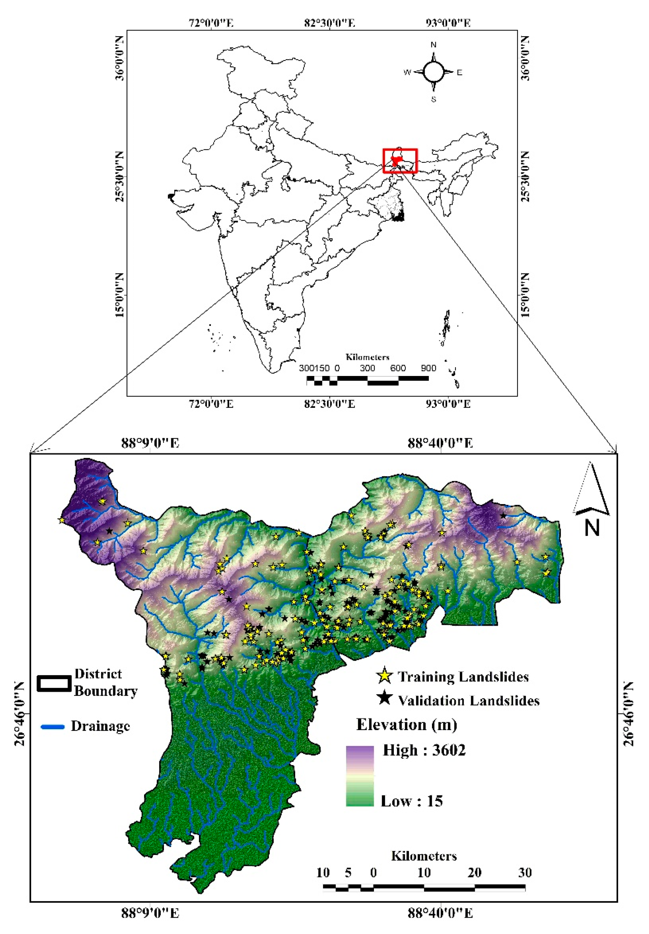
2.1. Study Area
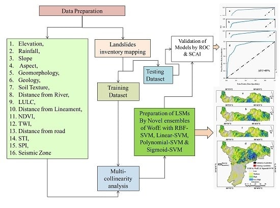
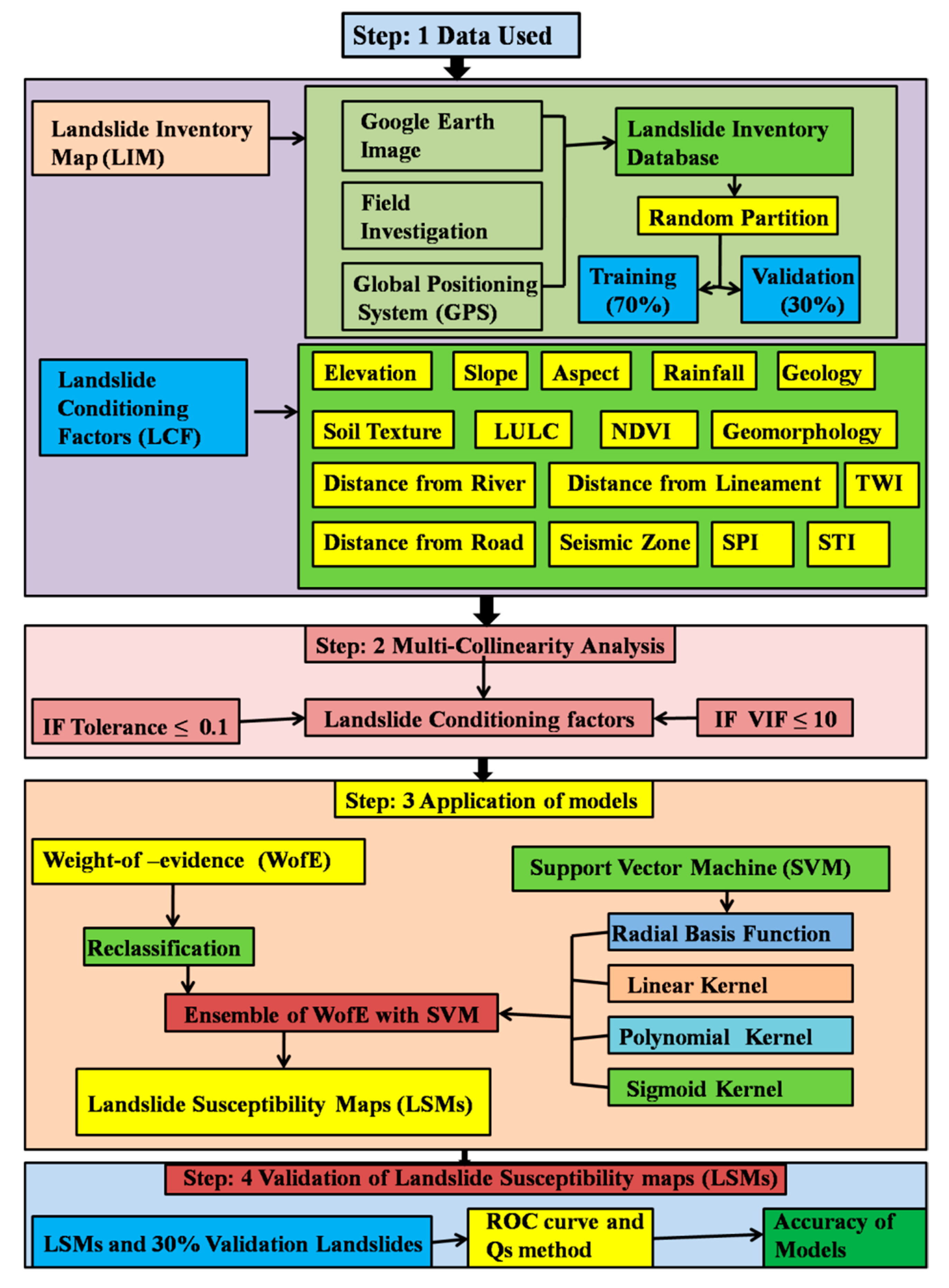
2.2. Methodology
2.3. Data Preparation
2.3.1. Landslide Inventory Dataset
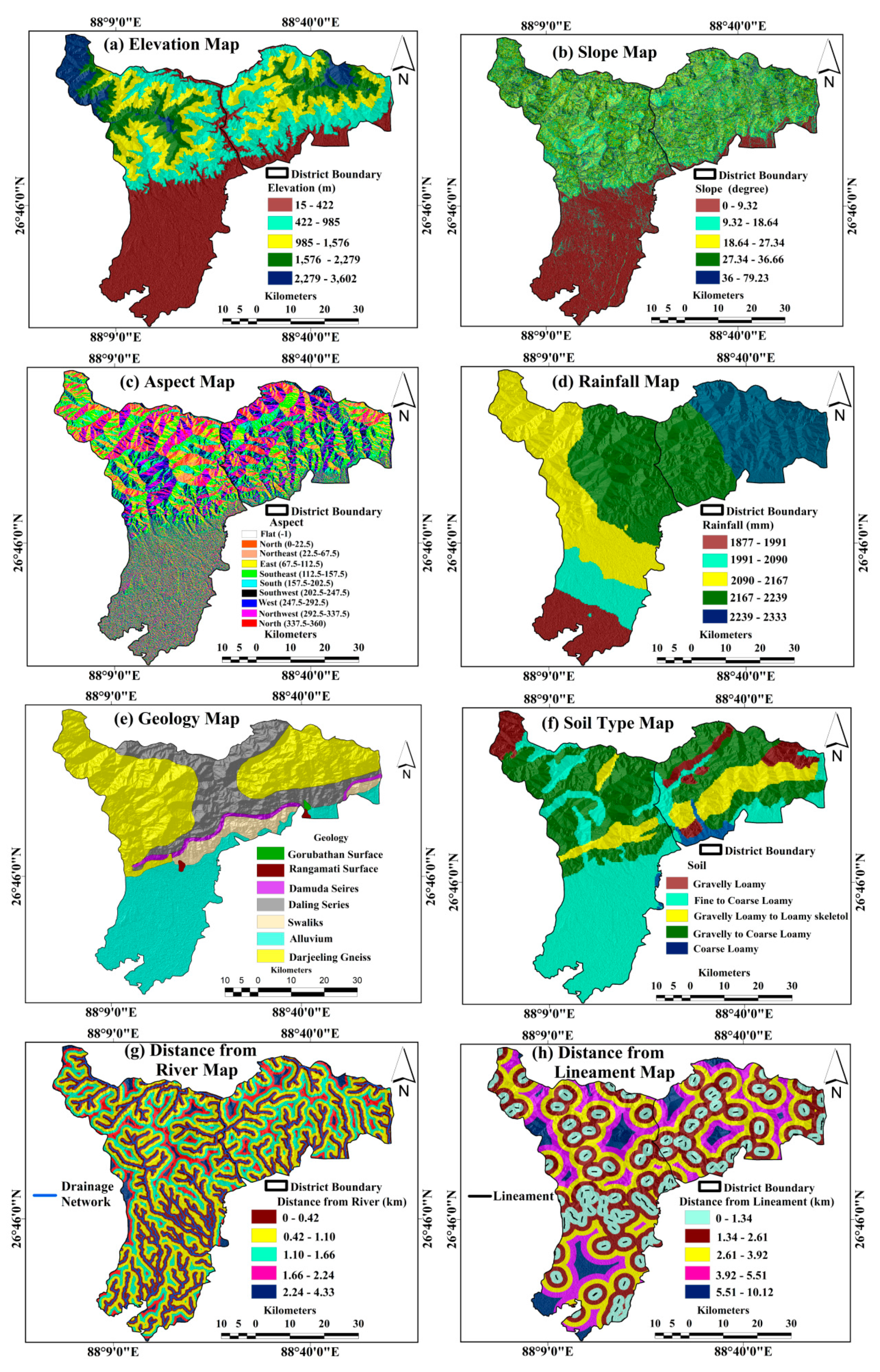
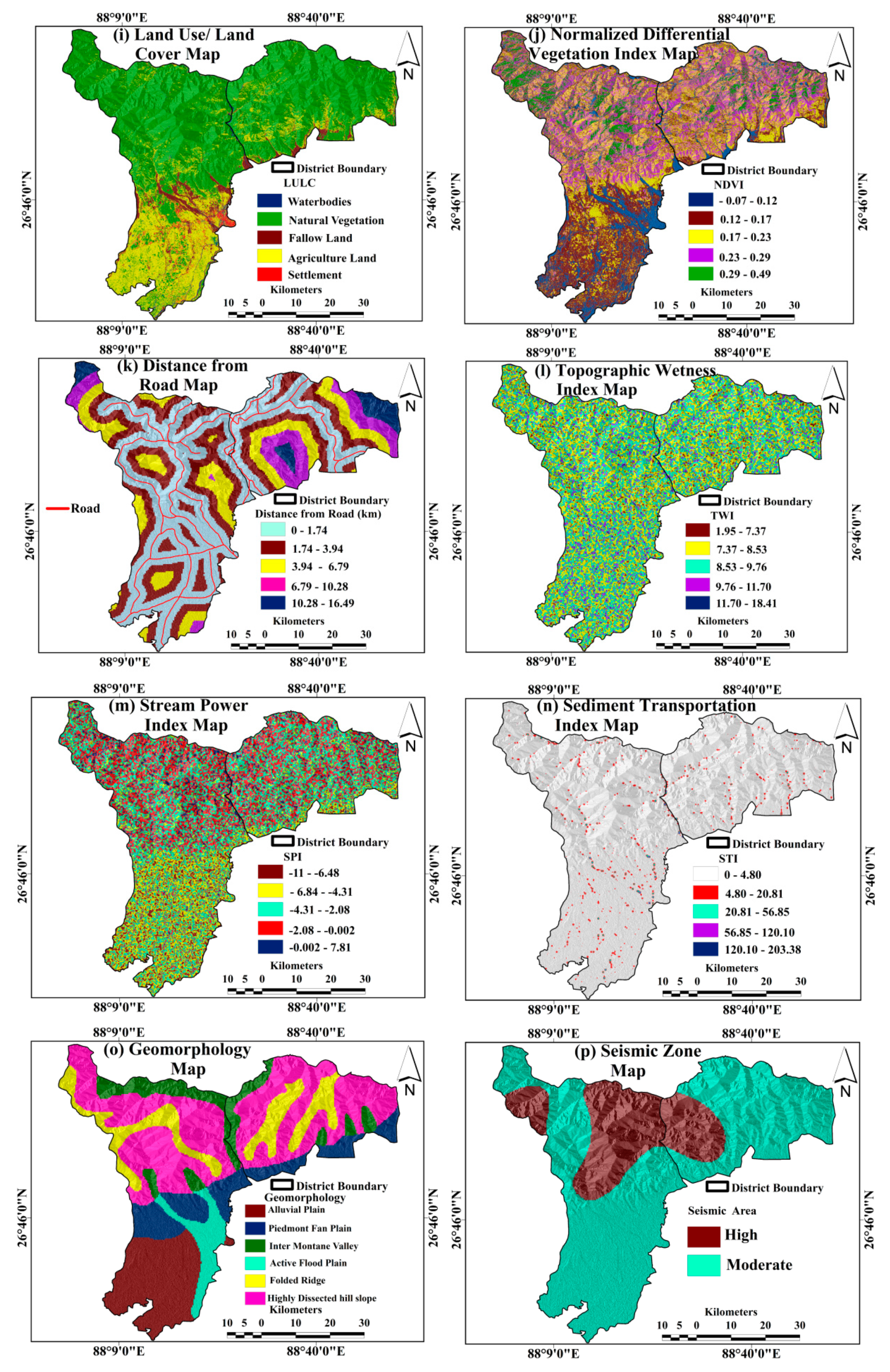
2.3.2. Preparing Effective Factors
2.4. Multicollinearity Analysis
2.5. Models
2.5.1. Weight-of-Evidence (WofE) Model
2.5.2. Support Vector Machine (SVM) Model
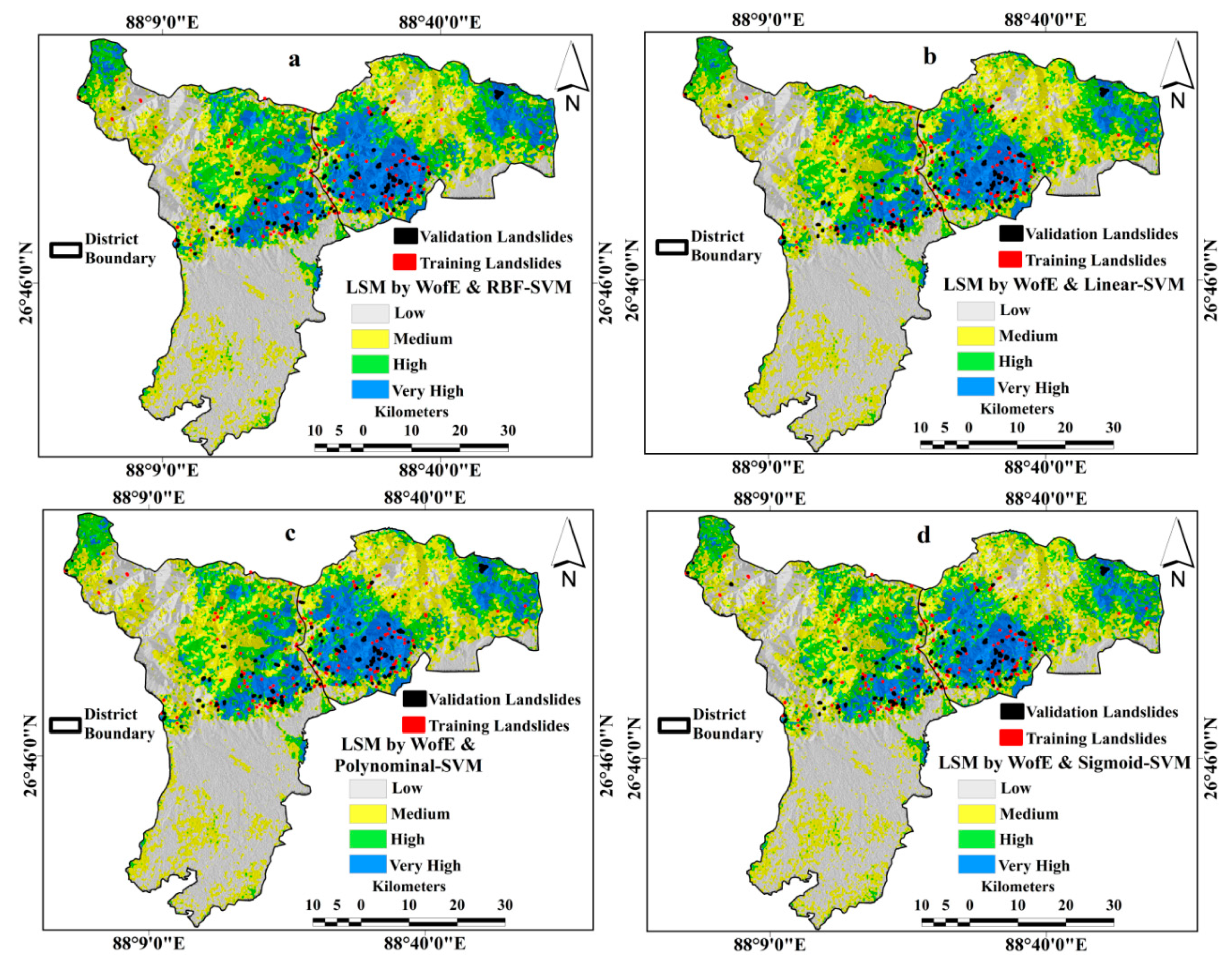
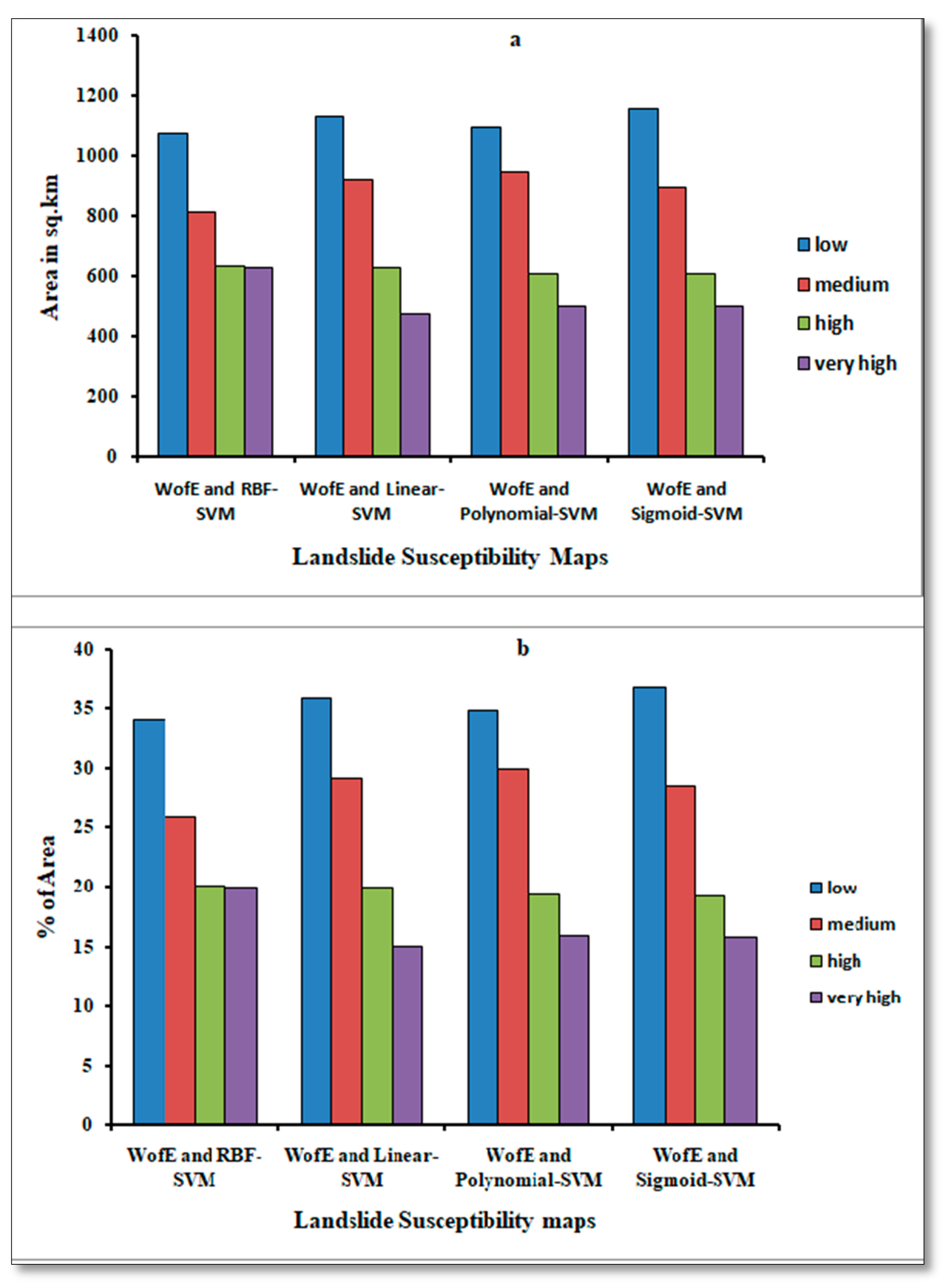
3.3. Landslide Susceptibility Models
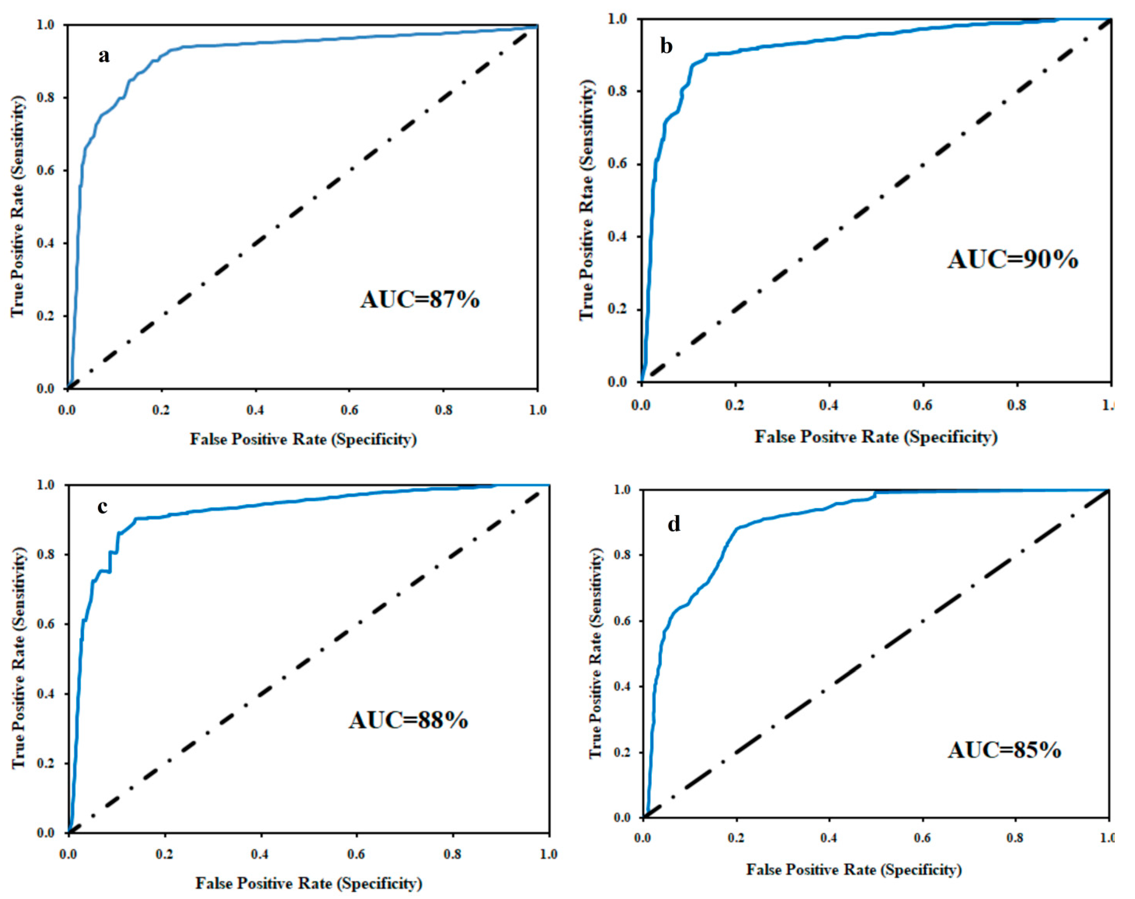
3.4. Validation and Comparison of Models
4. Discussion
5. Conclusions
Author Contributions
Funding
Conflicts of Interest
References
- Bui, D.T.; Tuan, T.A.; Klempe, H.; Pradhan, B.; Revhaug, I. Spatial prediction models for shallow landslide hazards: A comparative assessment of the efficacy of support vector machines, artificial neural networks, kernel logistic regression, and logistic model tree. Landslides 2015, 13, 361–378. [Google Scholar] [CrossRef]
- Cruden, D.M.; Varnes, D.J. Landslide Types and Processes, Transportation Research Board, U.S. National Academy of Sciences. Spec. Rep. 1996, 247, 36–75. [Google Scholar]
- Gerrard, J. The landslide hazard in the Himalayas: Geological control and human action. Geomorphology 1994, 10, 221–230. [Google Scholar] [CrossRef]
- Bhandari, R.K. Landslide hazard zonation: Some thoughts. In Co** with Natural Hazards: Indian Context; Valdiya, K.S., Ed.; Orient Longman: Hyderabad, India, 2004; pp. 134–152. [Google Scholar]
- Panikkar, S.V.; Subramanyan, V.A. geomorphic evaluation of the landslides around Dehradun and Mussoorie, Uttar Pradesh, India. Geomorphology 1996, 15, 169–181. [Google Scholar] [CrossRef]
- Sarkar, S. Landslides in Darjiling Himalayas. Trans. Jpn. Geomorphol. Union 1999, 20, 299–315. [Google Scholar]
- Fan, X.; Scaringi, G.; Domènech, G.; Yang, F.; Guo, X.; Dai, L.; Huang, R. Two multi-temporal datasets that track the enhanced landsliding after the 2008 Wenchuan earthquake. Earth Syst. Sci. Data 2019, 11, 35–55. [Google Scholar] [CrossRef]
- Yilmaz, I. Comparison of landslide susceptibility map** methodologies for Koyulhisar, Turkey: Conditional probability, logistic regression, artificial neural networks, and support vector machine. Environ. Earth Sci. 2009, 61, 821–836. [Google Scholar] [CrossRef]
- Abedini, M.; Ghasemyan, B.; Mogaddam, M.H.R. Landslide susceptibility map** in Bijar city, Kurdistan Province, Iran: A comparative study by logistic regression and AHP models. Environ. Earth Sci. 2017, 76, 308. [Google Scholar] [CrossRef]
- Regmi, A.D.; Devkota, K.C.; Yoshida, K.; Pradhan, B.; Pourghasemi, H.R.; Kumamoto, T.; Akgun, A. Application of frequency ratio, statistical index, and weights-of-evidence models and their comparison in landslide susceptibility map** in Central Nepal Himalaya. Arab. J. Geosci. 2013, 7, 725–742. [Google Scholar] [CrossRef]
- Chawla, A.; Pasupuleti, S.; Chawla, S.; Rao, A.C.S.; Sarkar, K.; Dwivedi, R. Landslide Susceptibility Zonation Map**: A Case Study from Darjeeling District, Eastern Himalayas, India. J. Indian Soc. Remote Sens. 2019, 47, 497–511. [Google Scholar] [CrossRef]
- Shahabi, H.; Hashim, M. Landslide susceptibility map** using GIS-based statistical models and Remote sensing data in tropical environment. Sci. Rep. 2015, 5, 15. [Google Scholar] [CrossRef] [PubMed]
- Roy, J.; Saha, S. Landslide susceptibility map** using knowledge driven statistical models in Darjeeling District, West Bengal, India. Geoenvironmental Disasters 2019, 6, 11. [Google Scholar] [CrossRef]
- Pradhan, B. A comparative study on the predictive ability of the decision tree, support vector machine and neuro-fuzzy models in landslide susceptibility map** using GIS. Comput. Geosci. 2013, 51, 350–365. [Google Scholar] [CrossRef]
- Pourghasemi, H.R.; Jirandeh, A.G.; Pradhan, B.; Xu, C.; Gokceoglu, C. Landslide susceptibility map** using support vector machine and GIS at the Golestan Province, Iran. J. Earth Syst. Sci. 2013, 122, 349–369. [Google Scholar] [CrossRef]
- Pham, B.T.; Pradhan, B.; Bui, D.T.; Prakash, I.; Dholakia, M. A comparative study of different machine learning methods for landslide susceptibility assessment: A case study of Uttarakhand area (India). Environ. Model. Softw. 2016, 84, 240–250. [Google Scholar] [CrossRef]
- Goetz, J.; Brenning, A.; Petschko, H.; Leopold, P. Evaluating machine learning and statistical prediction techniques for landslide susceptibility modeling. Comput. Geosci. 2015, 81, 1–11. [Google Scholar] [CrossRef]
- Gravina, T.; Figliozzi, E.; Mari, N.; Schinosa, F.D.L.T. Landslide risk perception in Frosinone (Lazio, Central Italy). Landslides 2016, 14, 1419–1429. [Google Scholar] [CrossRef]
- Pham, B.T.; Bui, D.T.; Prakash, I.; Dholakia, M. Hybrid integration of Multilayer Perceptron Neural Networks and machine learning ensembles for landslide susceptibility assessment at Himalayan area (India) using GIS. Catena 2017, 149, 52–63. [Google Scholar] [CrossRef]
- Pawde, M.B.; Saha, S.S. Geology of Darjeeling Himalaya; GSI: Kolkata, India, 1982. [Google Scholar]
- Pramanik, M.K. Site suitability analysis for agricultural land use of Darjeeling district using AHP and GIS techniques. Model. Earth Syst. Environ. 2016, 2. [Google Scholar] [CrossRef]
- Government of West Bengal. Bureau of Applied Economics and Statistics; Department of Statistics & Programme Implementation, District Statistical Handbook, Government of West Bengal: Kolkata, India, 2013.
- Guzzetti, F.; Reichenbach, P.; Ardizzone, F.; Cardinali, M.; Galli, M. Estimating the quality of landslide susceptibility models. Geomorphology 2006, 81, 166–184. [Google Scholar] [CrossRef]
- Li, Z.; Zhu, Q.; Gold, C. Digital Terrain Modeling: Principles and Methodology; CRC Press: Boca Raton, FL, USA, 2005. [Google Scholar]
- Wentworth, C.K. A simplified method of determining the average slope of land surfaces. Am. J. Sci. 1930, 117, 184–194. [Google Scholar] [CrossRef]
- Burrough, P.A.; McDonell, R.A. Principles of Geographical Information Systems; Oxford University Press: New York, NY, USA, 1998; p. 190. [Google Scholar]
- Bayraktar, H.; Turalioglu, S. A Kriging-based approach for locating a sampling site—In the assessment of air quality. Stoch. Environ. Res. Risk Assess. 2005, 19, 301–305. [Google Scholar] [CrossRef]
- Anderson, C.G.; Maxwell, D.C. Starting a Digitization Center; Elsevier: Amsterdam, The Netherlands, 2004; ISBN 978-1843340737. [Google Scholar]
- Ay, N.; Amari, S.-I. A Novel Approach to Canonical Divergences within Information Geometry. Entropy 2015, 17, 8111–8129. [Google Scholar] [CrossRef]
- Myung, I.J. Tutorial on Maximum Likelihood Estimation. J. Math. Psychol. 2003, 47, 90–100. [Google Scholar] [CrossRef]
- Crippen, R.E. Calculating the vegetation index faster. Remote Sens. Environ. 1990, 34, 71–73. [Google Scholar] [CrossRef]
- Moore, I.D.; Grayson, R.B.; Ladson, A.R. Digital terrain modelling: A review of hydrological, geomorphological, and biological applications. Hydrol. Process. 1991, 5, 3–30. [Google Scholar] [CrossRef]
- Moore, I.D.; Burch, G.J. Physical Basis of the Length Slope Factor in the Universal Soil Loss Equation. Soil Sci. Soc. Am. 1986, 50, 1294–1298. [Google Scholar] [CrossRef]
- Available online: http://dx.doi.org/10.2136/sssaj1986.03615995005000050042x (accessed on 21 October 2017).
- O’Brien, R.M. A Caution Regarding Rules of Thumb for Variance Inflation Factors. Qual. Quant. 2007, 41, 673–690. [Google Scholar] [CrossRef]
- Dormann, C.F.; Elith, J.; Bacher, S.; Buchmann, C.; Carl, G.; Carré, G.; Lautenbach, S. Collinearity: A review of methods to deal with it and a simulation study evaluating their performance. Ecography 2012, 36, 27–46. [Google Scholar] [CrossRef]
- Wang, H.; Wang, G.; Wang, F.; Sassa, K.; Chen, Y. Probabilistic modeling of seismically triggered landslides using Monte Carlo simulations. Landslide 2008, 5, 387–395. [Google Scholar] [CrossRef]
- Mohammady, M.; Pourghasemi, H.R.; Pradhan, B. Landslide susceptibility map** at Golestan Province, Iran: A comparison between frequency ratio, Dempster-Shafer, and weights-ofevidence models. J. Asian Earth Sci. 2012, 61, 221–236. [Google Scholar] [CrossRef]
- Bonham-Carter, G.F. Geographic information systems for geoscientists: Modeling with GIS. In Computer Methods in the Geosciences; Bonham-Carter, F., Ed.; Pergamon: Oxford, UK, 1994; p. 398. [Google Scholar]
- Dahal, R.K.; Hasegawa, S.; Nonomura, A.; Yamanaka, M.; Dhakal, S.; Paudyal, P. Predictive modeling of rainfall-induced landslide hazard in the Lesser Himalaya of Nepal based on weights-of evidence. Geomorphology 2008, 102, 496–510. [Google Scholar] [CrossRef]
- Dahal, R.K.; Hasegawa, S.; Nonomura, A.; Yamanaka, M.; Masuda, T.; Nishino, K. GIS-based weights-of-evidence modeling of rainfall-induced landslides in small catchments for landslide susceptibility map**. Environ. Geol. 2008, 54, 314–324. [Google Scholar] [CrossRef]
- Wan, S.; Lei, T.C. A knowledge-based decision support system to analyze the debris-flow problems at Chen-Yu-Lan River, Taiwan. Knowl. Based Syst. 2009, 22, 580–588. [Google Scholar] [CrossRef]
- Yao, X.; Tham, L.; Dai, F. Landslide susceptibility map** based on support vector machine: A case study on natural slopes of Hong Kong, China. Geomorphology 2008, 101, 572–582. [Google Scholar] [CrossRef]
- Marjanovic, M.; Kovacevic, M.; Bajat, B.; Vozenilek, V. Landslide susceptibility assessment using SVM machine learning algorithm. Eng. Geol. 2011, 123, 225–234. [Google Scholar] [CrossRef]
- Tehrany, M.S.; Pradhan, B.; Jebu, M.N. A comparative assessment between object and pixel-based classification approaches for land use/land cover map** using SPOT 5 imagery. Geocarto Int. 2013, 29, 1–19. [Google Scholar] [CrossRef]
- Tien Bui, D.; Pradhan, B.; Lofman, O.; Revhaug, I. Landslide susceptibility assessment in Vietnam using support vector machines, decision tree, and Naïve Bayes Models. Math. Probl. Eng. 2012, 2012, 1–26. [Google Scholar] [CrossRef] [Green Version]
- Cortes, C.; Vapnik, V. Support-vector networks. Mach. Learn. 1995, 20, 273–297. [Google Scholar] [CrossRef]
- Samui, P. Slope stability analysis: A support vector machine approach. Environ. Geol. 2008, 56, 255–267. [Google Scholar] [CrossRef]
- Arabameri, A.; Pradhan, B.; Rezaei, K. Gully erosion zonation map** using integrated geographically weighted regression with certainty factor and random forest models in GIS. J. Environ. Manag. 2019, 232, 928–942. [Google Scholar] [CrossRef]
- Arabameri, A.; Pradhan, B.; Rezaei, K. Spatial prediction of gully erosion using ALOS PALSAR data and ensemble bivariate and data mining models. Geosci. J. 2019, 23, 1–18. [Google Scholar] [CrossRef]
- Arabameri, A.; Cerda, A.; Tiefenbacher, J.P. Spatial pattern analysis and prediction of gully erosion using novel hybrid model of entropy-weight of evidence. Water 2019, 11, 1129. [Google Scholar] [CrossRef] [Green Version]
- Arabameri, A.; Pradhan, B.; Rezaei, K.; Conoscenti, C. Gully erosion susceptibility map** using GISbased multi-criteria decision analysis techniques. Catena 2019, 180, 282–297. [Google Scholar] [CrossRef]
- Arabameri, A.; Rezaei, K.; Cerda, A.; Lombardo, L.; Rodrigo-Comino, J. GIS-based groundwater potential map** in Shahroud plain, Iran. A comparison among statistical (bivariate and multivariate), data mining and MCDM approaches. Sci. Total Environ. 2019, 658, 160–177. [Google Scholar] [CrossRef]
- Arabameri, A.; Pourghasemi, H.R.; Yamani, M. Applying different scenarios for landslide spatial modeling using computational intelligence methods. Environ. Earth Sci. 2017, 76, 832. [Google Scholar] [CrossRef]
- Arabameri, A.; Pradhan, B.; Rezaei, K.; Sohrabi, M.; Kalantari, Z. GIS-based landslide susceptibility map** using numerical risk factor bivariate model and its ensemble with linear multivariate regression and boosted regression tree algorithms. J. Mt. Sci. 2019, 16, 595–618. [Google Scholar] [CrossRef]
- Arabameri, A.; Pradhan, B.; Rezaei, K.; Saro, L.; Sohrabi, M. An ensemble model for landslide susceptibility map** in a forested area. Geochem. Int. 2019, 1–18. [Google Scholar] [CrossRef]
- Chung, C.J.F.; Fabbri, A.G. Validation of Spatial Prediction Models for Landslide Hazard Map**. Nat. Hazards 2003, 30, 451–472. [Google Scholar] [CrossRef]
- Negnevitsky, M. Artificial Intelligence—A Guide to Intelligent Systems; Addison-Wesley Co.: Boston, MA, USA, 2002; p. 394. [Google Scholar]
- Mallick, J.; Singh, R.K.; Alawadh, M.A.; Islam, S.; Khan, R.A.; Qureshi, M.N. GIS-based landslide susceptibility evaluation using fuzzy-AHP multi-criteria decision-making techniques in the Abha Watershed, Saudi Arabia. Environ. Earth Sci. 2018, 77, 276. [Google Scholar] [CrossRef]
- Feizizadeh, B.; Roodposhti, M.S.; Jankowski, P.; Blaschke, T. A GIS-based extended fuzzy multi-criteria evaluation for landslide susceptibility map**. Comput. Geosci. 2014, 73, 208–221. [Google Scholar] [CrossRef] [PubMed] [Green Version]
- Park, S.; Choi, C.; Kim, B.; Kim, J. Landslide susceptibility map** using frequency ratio, analytic hierarchy process, logistic regression, and artificial neural network methods at the Inje area, Korea. Environ. Earth Sci. 2012, 68, 1443–1464. [Google Scholar] [CrossRef]
- Bijukchhen, S.M.; Kayastha, P.; Dhital, M.R. A comparative evaluation of heuristic and bivariate statistical modelling for landslide susceptibility map**s in Ghurmi–DhadKhola, east Nepal. Arab. J. Geosci. 2012, 6, 2727–2743. [Google Scholar] [CrossRef]
- Pradhan, B.; Youssef, A.M. Manifestation of remote sensing data and GIS on landslide hazard analysis using spatial-based statistical models. Arab. J. Geosci. 2009, 3, 319–326. [Google Scholar] [CrossRef]
- Ozdemir, A.; Altural, T. A comparative study of frequency ratio, weights of evidence and logistic regression methods for landslide susceptibility map**: Sultan Mountains, SW Turkey. J. Asian Earth Sci. 2013, 64, 180–197. [Google Scholar] [CrossRef]
- Arabameri, A.; Yamani, M.; Pradhan, B.; Melesse, A.; Shirani, K.; Bui, D.T. Novel ensembles of COPRAS multi-criteria decision-making with logistic regression, boosted regression tree, and random forest for spatial prediction of gully erosion susceptibility. Sci. Total Environ. 2019, 688, 903–916. [Google Scholar] [CrossRef]
- Tien Bui, D.; Hoang, N.D.; Martínez-Álvarez, F.; Ngo, P.T.T.; Hoa, P.V.; Pham, T.D.; Samui, P.; Costache, R. A novel deep learning neural network approach for predicting flash flood susceptibility: A case study at a high frequency tropical storm area. Sci. Total Environ. 2019. [Google Scholar] [CrossRef]
- Abedini, M.; Tulabi, S. Assessing LNRF, FR, and AHP models in landslide susceptibility map** index: A comparative study of Nojian watershed in Lorestan province, Iran. Environ. Earth Sci. 2018, 77, 405. [Google Scholar] [CrossRef]
- Haneberg, W.C.; Cole, W.F.; Kasali, G. High-resolution lidar-based landslide hazard map** and modeling, UCSF Parnassus Campus, San Francisco, USA. Bull. Eng. Geol. Environ. 2009, 68, 263–276. [Google Scholar] [CrossRef]
- Nichol, J.E.; Shaker, A.; Wong, M.S. Application of high-resolution stereo satellite images to detailed landslide hazard assessment. Geomorphology 2006, 76, 68–75. [Google Scholar] [CrossRef]


| Age | Series | Lithological Characteristics |
|---|---|---|
| Recent (Holocene) Pleistocene | Sub-aerial formations (soil, alluvia, colluvial) Raised Terraces | Younger flood plain deposits of the rivers composed of sand, gravel, pebble, etc. and soil covering the rocks sandy, clay, gravel, pebble, boulders etc. representing older fluvial deposits |
| Miocene | Siwalik | Micaceous sandstones with slaty bands, seams of graphitic coal, silts and minor bands of limestone |
| Permian | Damuda Series (Lower Gondwana) | Quartzitic sandstones with slaty bands, carbonaceous shales, seams of graphitic coal, lamprophyre sills and minor bands of limestone |
| Precambrian | 1) Darjeeling gneiss 2) Daling gneiss | Golden-silvery micaschists; Carbonaceousmicaschists; Granatiferousmicaschists and coarse grained gneisses. Slates (greenish to grey with perfect slaty cleavage). Phyllites surrounded by pebbles of quartz, Chlorite-schists with bands of grilty schist’s injected with gneiss (crinkled). Granites, pagmatites’s and quartz veins, with tourmaline and iron as accessories |
| Sl. No. | Parameters | Data Used & Scale | Sources of Data Types | Techniques | References |
|---|---|---|---|---|---|
| 1 | Elevation | DEM 30 m × 30 | U.S Geological Survey | 30 m × 30 m digital elevation model | [24] |
| 2 | Slope | DEM 30 m × 30 | U.S Geological Survey | N=No. of Contour Cutting; i=Contour Interval | [25] |
| 3 | Aspect | DEM 30 m × 30 | U.S Geological Survey | Where, dz/dx= ((c+2f+i)−(a+2d+g))/8 dz/dy=((g+2h+i)−(a+2b+c))/8 Here, a to i indicates the cell value of 3*3 window. | [26] |
| 4 | Rainfall | Annual average rainfall data of different stations in the last 5 years | Indian Metrological Department (IMD) | Kriging Interpolation method | [27] |
| 5 | Geology | Reference geological map 1: 50,000 | Geological Survey of India | Digitization process | [28] |
| 6 | Soil | Reference district soil map 1: 50,000 | National Bureau of Soil Survey and Land Use Planning | Digitization process | [28] |
| 7 | Distance from River | Reference Topomap 1: 50,000 | Survey of India | Euclidian Distance Buffering | [29] |
| 8 | Distance from Lineament | Reference sheet of Lineament 30 m × 30 | “https://bhuvan-vec2.nrsc.gov.in/bhuvan/wms” | Euclidian Distance Buffering | [29] |
| 9 | Land use/land cover (LULC) | Landsat 8 OLI/TIRS 30 m × 30 | U.S Geological Survey | Maximum likelihood Classification | [30] |
| 10 | Normalized differential vegetation index (NDVI) | Landsat 8 OLI/TIRS 30 m × 30 | U.S Geological Survey | Where NIR is the near infrared band or band 4 and IR is the infrared band or band 3. | [31] |
| 11 | Distance from road | Reference Topomap 1: 50,000 | Survey of India | Euclidian Distance Buffering | [29] |
| 12 | Topographic wetness index (TWI) | DEM 30 m×30 1: 50,000 | U.S Geological Survey | Where α is the cumulative upslope area draining through a point (per unit contour length), and β is the slope gradient (in degree). | [32]. |
| 13 | Stream power index (SPI) | DEM 30 m × 30 1: 50,000 | U.S Geological Survey | Where AS is the upstream contributing area and β is the slope gradient (in degrees) | [32]. |
| 14 | Sediment transportation index (STI) | DEM 30 m × 30 | U.S Geological Survey | Where, As, is the specific catchment area; ‘B’ is the local slope gradient in degrees; m is usually set to 0.4, ‘n’, is usually set to 0.0896 | [33] |
| 15 | Geomorphology | Reference sheet 1: 50,000 | “https://bhuvan-vec2.nrsc.gov.in/bhuvan/wms” | Digitization process | [27] |
| 16 | Seismic zone map | Last 200 years point data of earthquake 30 m × 30 | National Centre for Seismology, New Delhi, India | Gridding and Interpolation (Inverse distance weight method) | [11] |
| Kernel Types | Equations | Kernel Parameters |
|---|---|---|
| Radial Basis Function (RBF) | ||
| Linear kernel | --- | |
| Polynomial kernel | ||
| Sigmoid kernel |
| Landslide Conditioning Factors | Collinearity Statistics | |
|---|---|---|
| Tolerance | VIF | |
| Rainfall | 0.446 | 2.241 |
| Elevation | 0.520 | 1.924 |
| Slope | 0.824 | 1.213 |
| Aspect | 0.672 | 1.488 |
| Geology | 0.688 | 1.453 |
| Soil | 0.756 | 1.323 |
| Distance from River | 0.570 | 1.753 |
| Distance from lineament | 0.773 | 1.294 |
| Distance from Road | 0.499 | 2.003 |
| Land use/land cover (LULC) | 0.754 | 1.326 |
| Normalized differential vegetation index (NDVI) | 0.757 | 1.320 |
| Topographic wetness index (TWI) | 0.677 | 1.477 |
| Stream power index (SPI) | 0.684 | 1.461 |
| Sediment transportation index (STI) | 0.768 | 1.302 |
| Geomorphology | 0.789 | 1.268 |
| Seismic zone | 0.618 | 1.618 |
| Rainfall (mm) | Pixels | % of Pixels | Landslide Pixels | % of Pixels | W+ | W− | C | S2W+ | S2W− | S© | W |
|---|---|---|---|---|---|---|---|---|---|---|---|
| 1877.38–1991.97 | 322590 | 8.784 | 0 | 0.000 | 0.000 | 0.092 | 0.000 | 0.000 | 0.000 | 0.000 | 0.000 |
| 1991.97–2090.54 | 289906 | 7.894 | 0 | 0.000 | 0.000 | 0.082 | 0.000 | 0.000 | 0.000 | 0.000 | 0.000 |
| 2090.45–2167.44 | 944320 | 25.712 | 393 | 7.895 | −1.182 | 0.215 | −1.397 | 0.003 | 0.000 | 0.053 | −26.580 |
| 2167.44–2239.06 | 1333493 | 36.309 | 3670 | 73.684 | 0.709 | −0.885 | 1.594 | 0.000 | 0.001 | 0.032 | 49.504 |
| 2239.06–2333.96 | 782357 | 21.302 | 918 | 18.421 | −0.145 | 0.036 | −0.182 | 0.001 | 0.000 | 0.037 | −4.963 |
| Slope (Degree) | |||||||||||
| 0–9.32 | 1175818 | 32.015 | 92 | 1.847 | −2.854 | 0.368 | −3.222 | 0.011 | 0.000 | 0.105 | −30.614 |
| 9.32–18.64 | 665098 | 18.109 | 571 | 11.464 | −0.458 | 0.078 | −0.536 | 0.002 | 0.000 | 0.044 | −12.044 |
| 18.44–27.34 | 813896 | 22.161 | 1172 | 23.529 | 0.060 | −0.018 | 0.078 | 0.001 | 0.000 | 0.033 | 2.326 |
| 27.34–36.66 | 694449 | 18.909 | 1579 | 31.700 | 0.518 | −0.172 | 0.690 | 0.001 | 0.000 | 0.030 | 22.622 |
| 36.66–79.23 | 323404 | 8.806 | 1567 | 31.460 | 1.277 | −0.286 | 1.563 | 0.001 | 0.000 | 0.031 | 51.122 |
| Altitude(m) | |||||||||||
| 15–422 | 1351511 | 36.799 | 417 | 8.373 | −1.482 | 0.372 | −1.854 | 0.002 | 0.000 | 0.051 | −36.226 |
| 422 – 985 | 837224 | 22.796 | 2491 | 50.000 | 0.787 | −0.435 | 1.222 | 0.000 | 0.000 | 0.028 | 43.079 |
| 985 –1576 | 738499 | 20.108 | 1005 | 20.173 | 0.003 | −0.001 | 0.004 | 0.001 | 0.000 | 0.035 | 0.115 |
| 1576 – 2279 | 518669 | 14.122 | 839 | 16.844 | 0.176 | −0.032 | 0.209 | 0.001 | 0.000 | 0.038 | 5.509 |
| 2279 – 3602 | 226762 | 6.174 | 230 | 4.610 | −0.293 | 0.017 | −0.309 | 0.004 | 0.000 | 0.068 | −4.572 |
| Aspect | |||||||||||
| Flat(−1) | 1905 | 0.052 | 0 | 0.000 | 0.000 | 0.001 | 0.000 | 0.000 | 0.000 | 0.000 | 0.000 |
| north | 236967 | 6.452 | 39 | 0.788 | −2.104 | 0.059 | −2.163 | 0.025 | 0.000 | 0.160 | −13.495 |
| northeast | 462023 | 12.580 | 363 | 7.289 | −0.546 | 0.059 | −0.605 | 0.003 | 0.000 | 0.055 | −11.098 |
| east | 454970 | 12.388 | 651 | 13.061 | 0.053 | −0.008 | 0.061 | 0.002 | 0.000 | 0.042 | 1.443 |
| southeast | 522200 | 14.219 | 1098 | 22.045 | 0.439 | −0.096 | 0.535 | 0.001 | 0.000 | 0.034 | 15.640 |
| south | 525807 | 14.317 | 1292 | 25.946 | 0.596 | −0.146 | 0.742 | 0.001 | 0.000 | 0.032 | 22.922 |
| southwest | 457236 | 12.450 | 890 | 17.868 | 0.362 | −0.064 | 0.426 | 0.001 | 0.000 | 0.037 | 11.505 |
| west | 378362 | 10.302 | 462 | 9.279 | −0.105 | 0.011 | −0.116 | 0.002 | 0.000 | 0.049 | −2.376 |
| northwest | 419573 | 11.424 | 154 | 3.093 | −1.308 | 0.090 | −1.398 | 0.006 | 0.000 | 0.082 | −17.074 |
| north | 213621 | 5.817 | 31 | 0.630 | −2.223 | 0.054 | −2.277 | 0.032 | 0.000 | 0.179 | −12.718 |
| Geology | |||||||||||
| Swaliks | 1936266 | 52.721 | 3182 | 63.889 | 0.192 | −0.270 | 0.462 | 0.000 | 0.001 | 0.030 | 15.659 |
| Darjeeling Gneiss | 270526 | 7.366 | 692 | 13.889 | 0.635 | −0.073 | 0.709 | 0.001 | 0.000 | 0.041 | 17.273 |
| Daling series | 131471 | 3.580 | 415 | 8.333 | 0.847 | −0.051 | 0.897 | 0.002 | 0.000 | 0.051 | 17.480 |
| Alluvium | 678512 | 18.475 | 0 | 0.000 | 0.000 | 0.205 | 0.000 | 0.000 | 0.000 | 0.000 | 0.000 |
| Damuda series | 655890 | 17.859 | 692 | 13.889 | −0.252 | 0.047 | −0.299 | 0.001 | 0.000 | 0.041 | −7.293 |
| Soil | |||||||||||
| Gravelly-loamy | 274651 | 7.478 | 830 | 16.667 | 0.803 | −0.105 | 0.908 | 0.001 | 0.000 | 0.038 | 23.845 |
| Fine loamy_Coarse Loamy | 1477848 | 40.239 | 1107 | 22.222 | −0.594 | 0.264 | −0.858 | 0.001 | 0.000 | 0.034 | −25.171 |
| Gravelly loamy_LoamySkeletol | 450035 | 12.254 | 1107 | 22.222 | 0.596 | −0.121 | 0.717 | 0.001 | 0.000 | 0.034 | 21.019 |
| Gravelly Loamy_Coarse Loamy | 1404794 | 38.250 | 1660 | 33.333 | −0.138 | 0.077 | −0.214 | 0.001 | 0.000 | 0.030 | −7.131 |
| Coarse Loamy | 65336 | 1.779 | 277 | 5.556 | 1.142 | −0.039 | 1.181 | 0.004 | 0.000 | 0.062 | 19.055 |
| Distance from River (km) | |||||||||||
| 0–0.42 | 1160959 | 31.611 | 1049 | 21.053 | −0.407 | 0.144 | −0.551 | 0.001 | 0.000 | 0.035 | −15.837 |
| 0.42–1.10 | 1291696 | 35.171 | 1966 | 39.474 | 0.116 | −0.069 | 0.184 | 0.001 | 0.000 | 0.029 | 6.356 |
| 1.10–1.66 | 750401 | 20.432 | 1442 | 28.947 | 0.349 | −0.113 | 0.462 | 0.001 | 0.000 | 0.031 | 14.784 |
| 1.66–2.26 | 371677 | 10.120 | 393 | 7.895 | −0.249 | 0.024 | −0.273 | 0.003 | 0.000 | 0.053 | −5.195 |
| 2.26–4.33 | 97931 | 2.666 | 131 | 2.632 | −0.013 | 0.000 | −0.014 | 0.008 | 0.000 | 0.089 | −0.153 |
| Distance from Lineament(km) | |||||||||||
| 0–1.54 | 763490 | 20.788 | 906 | 18.182 | −0.134 | 0.032 | −0.167 | 0.001 | 0.000 | 0.037 | −4.531 |
| 1.54–2.85 | 1093457 | 29.773 | 1019 | 20.455 | −0.376 | 0.125 | −0.501 | 0.001 | 0.000 | 0.035 | −14.243 |
| 2.85–4.20 | 941314 | 25.630 | 1472 | 29.545 | 0.142 | −0.054 | 0.197 | 0.001 | 0.000 | 0.031 | 6.323 |
| 4.20–5.75 | 633142 | 17.239 | 1245 | 25.000 | 0.372 | −0.099 | 0.471 | 0.001 | 0.000 | 0.033 | 14.378 |
| 5.75–10.12 | 241263 | 6.569 | 340 | 6.818 | 0.037 | −0.003 | 0.040 | 0.003 | 0.000 | 0.056 | 0.710 |
| Distance from Road(km) | |||||||||||
| 0–1.74 | 1636028 | 44.546 | 792 | 15.909 | −1.031 | 0.417 | −1.448 | 0.001 | 0.000 | 0.039 | −37.353 |
| 1.74–3.94 | 988335 | 26.911 | 906 | 18.182 | −0.393 | 0.113 | −0.506 | 0.001 | 0.000 | 0.037 | −13.754 |
| 3.94–6.72 | 589253 | 16.044 | 906 | 18.182 | 0.125 | −0.026 | 0.151 | 0.001 | 0.000 | 0.037 | 4.109 |
| 6.72–10.22 | 316628 | 8.621 | 1472 | 29.545 | 1.235 | −0.260 | 1.495 | 0.001 | 0.000 | 0.031 | 48.066 |
| 10.22–16.49 | 142420 | 3.878 | 906 | 18.182 | 1.550 | −0.161 | 1.711 | 0.001 | 0.000 | 0.037 | 46.466 |
| Land use/Land cover | |||||||||||
| Water bodies | 40427 | 1.101 | 0 | 0.000 | 0.000 | 0.011 | 0.000 | 0.000 | 0.000 | 0.000 | 0.000 |
| Vegetation | 2650294 | 72.163 | 1119 | 22.464 | −1.168 | 1.027 | −2.195 | 0.001 | 0.000 | 0.034 | −64.607 |
| Fallow land | 168382 | 4.585 | 1624 | 32.609 | 1.970 | −0.348 | 2.318 | 0.001 | 0.000 | 0.030 | 76.445 |
| Agricultural land | 763256 | 20.782 | 2238 | 44.928 | 0.773 | −0.364 | 1.137 | 0.000 | 0.000 | 0.029 | 39.858 |
| Settlement | 50306 | 1.370 | 0 | 0.000 | 0.000 | 0.014 | 0.000 | 0.000 | 0.000 | 0.000 | 0.000 |
| Normalized differential vegetation index (NDVI) | |||||||||||
| −0.07–0.12 | 442450 | 12.047 | 1399 | 28.093 | 0.849 | −0.202 | 1.050 | 0.001 | 0.000 | 0.032 | 33.271 |
| 0.12–0.17) | 972514 | 26.480 | 1421 | 28.523 | 0.074 | −0.028 | 0.103 | 0.001 | 0.000 | 0.031 | 3.270 |
| 0.17–0.23) | 997257 | 27.154 | 1312 | 26.336 | −0.031 | 0.011 | −0.042 | 0.001 | 0.000 | 0.032 | −1.297 |
| 0.23–0.29 | 816592 | 22.234 | 618 | 12.411 | −0.584 | 0.119 | −0.703 | 0.002 | 0.000 | 0.043 | −16.346 |
| 0.29–0.49 | 443851 | 12.085 | 231 | 4.636 | −0.959 | 0.081 | −1.041 | 0.004 | 0.000 | 0.067 | −15.436 |
| Topographic wetness index (TWI) | |||||||||||
| 1.95–7.37 | 582990 | 15.874 | 918 | 18.421 | 0.149 | −0.031 | 0.180 | 0.001 | 0.000 | 0.037 | 4.916 |
| 7.37–8.53 | 1326854 | 36.128 | 2097 | 42.105 | 0.153 | −0.098 | 0.252 | 0.000 | 0.000 | 0.029 | 8.765 |
| 8.53–9.76 | 1088701 | 29.643 | 1311 | 26.316 | −0.119 | 0.046 | −0.165 | 0.001 | 0.000 | 0.032 | −5.140 |
| 9.76–11.70 | 547267 | 14.901 | 655 | 13.158 | −0.125 | 0.020 | −0.145 | 0.002 | 0.000 | 0.042 | −3.454 |
| 11.70–18.91 | 126853 | 3.454 | 0 | 0.000 | 0.000 | 0.035 | 0.000 | 0.000 | 0.000 | 0.000 | 0.000 |
| Sediment transportation index (STI) | |||||||||||
| 0–4.80 | 3576809 | 97.390 | 4850 | 97.368 | 0.000 | 0.008 | −0.008 | 0.000 | 0.008 | 0.089 | −0.096 |
| 4.80–20.81 | 78362 | 2.134 | 131 | 2.632 | 0.210 | −0.005 | 0.215 | 0.008 | 0.000 | 0.089 | 2.429 |
| 20.81–56.85 | 13728 | 0.374 | 0 | 0.000 | 0.000 | 0.004 | 0.000 | 0.000 | 0.000 | 0.000 | 0.000 |
| 56.85–120.10 | 3037 | 0.083 | 0 | 0.000 | 0.000 | 0.001 | 0.000 | 0.000 | 0.000 | 0.000 | 0.000 |
| 120.10–203.38 | 729 | 0.020 | 0 | 0.000 | 0.000 | 0.000 | 0.000 | 0.000 | 0.000 | 0.000 | 0.000 |
| Stream power index (SPI) | |||||||||||
| −11.16 – −6.84 | 457701 | 12.462 | 427 | 8.571 | −0.375 | 0.044 | −0.418 | 0.002 | 0.000 | 0.051 | −8.260 |
| −6.84 – −4.31 | 670452 | 18.255 | 1139 | 22.857 | 0.225 | −0.058 | 0.283 | 0.001 | 0.000 | 0.034 | 8.385 |
| −4.31 – −2.08 | 994622 | 27.082 | 1139 | 22.857 | −0.170 | 0.056 | −0.226 | 0.001 | 0.000 | 0.034 | −6.700 |
| −2.08 – −0.002 | 1003492 | 27.323 | 1423 | 28.571 | 0.045 | −0.017 | 0.062 | 0.001 | 0.000 | 0.031 | 1.978 |
| −0.002 – 7.81 | 546398 | 14.877 | 854 | 17.143 | 0.142 | −0.027 | 0.169 | 0.001 | 0.000 | 0.038 | 4.491 |
| Geomorphology | |||||||||||
| Alluvial plain | 591694 | 16.111 | 0 | 0.000 | 0.000 | 0.176 | 0.000 | 0.000 | 0.000 | 0.000 | 0.000 |
| Piedmont fan plain | 453016 | 12.335 | 119 | 2.381 | −1.646 | 0.108 | −1.754 | 0.008 | 0.000 | 0.093 | −18.867 |
| Inter montane valley | 383190 | 10.434 | 474 | 9.524 | −0.091 | 0.010 | −0.101 | 0.002 | 0.000 | 0.048 | −2.101 |
| Active flood plain | 205950 | 5.608 | 0 | 0.000 | 0.000 | 0.058 | 0.000 | 0.000 | 0.000 | 0.000 | 0.000 |
| Folded ridge | 499607 | 13.603 | 1067 | 21.429 | 0.455 | −0.095 | 0.550 | 0.001 | 0.000 | 0.035 | 15.919 |
| Highly dissected hill slope | 1539208 | 41.910 | 3321 | 66.667 | 0.465 | −0.556 | 1.021 | 0.000 | 0.001 | 0.030 | 33.948 |
| Seismic zone map | |||||||||||
| High | 1000641 | 27.246 | 2604 | 52.273 | 0.653 | −0.422 | 1.075 | 0.000 | 0.000 | 0.028 | 37.859 |
| Moderate | 2672024 | 72.754 | 2377 | 47.727 | −0.422 | 0.653 | −1.075 | 0.000 | 0.000 | 0.028 | −37.859 |
| Landslide Susceptibility Classes | WofE& RBF-SVM | WofE&Linear-SVM | WofE& Polynomial-SVM | WofE& Sigmoid-SVM | ||||
|---|---|---|---|---|---|---|---|---|
| Area in sq.km | % of Area | Area in sq.km | % of Area | Area in sq.km | % of Area | Area in sq.km | % of Area | |
| Low | 1071 | 34.0 | 1128 | 35.8 | 1095 | 34.8 | 1153 | 36.6 |
| Medium | 813 | 25.8 | 918 | 29.1 | 944 | 30.0 | 893 | 28.3 |
| High | 635 | 20.2 | 630 | 20.0 | 608 | 19.3 | 605 | 19.2 |
| Very High | 630 | 20.0 | 474 | 15.0 | 501 | 15.9 | 498 | 15.8 |
| Ensemble Models | Classes | ai (sq.km) | si (sq.km) | DR | s | Qs |
|---|---|---|---|---|---|---|
| WofE& RBF-SVM | Low | 1071.23 | 0.00 | 0.00 | 0.34 | 2.10 |
| Medium | 812.95 | 0.12 | 0.10 | 0.26 | ||
| High | 635.02 | 0.93 | 1.07 | 0.20 | ||
| Very High | 629.80 | 3.26 | 3.78 | 0.20 | ||
| WofE& Linear-SVM | Low | 1127.55 | 0.00 | 0.00 | 0.36 | 2.24 |
| Medium | 917.57 | 0.34 | 0.27 | 0.29 | ||
| High | 630.04 | 1.13 | 1.32 | 0.20 | ||
| Very High | 473.84 | 2.84 | 4.37 | 0.15 | ||
| WofE& Polynomial-SVM | Low | 1095.14 | 0.00 | 0.00 | 0.35 | 2.10 |
| Medium | 944.15 | 0.34 | 0.26 | 0.30 | ||
| High | 608.44 | 1.13 | 1.36 | 0.19 | ||
| Very High | 501.27 | 2.84 | 4.13 | 0.16 | ||
| WofE& Sigmoid-SVM | Low | 1153.40 | 0.00 | 0.00 | 0.37 | 2.18 |
| Medium | 892.57 | 0.23 | 0.19 | 0.28 | ||
| High | 604.55 | 1.25 | 1.51 | 0.19 | ||
| Very High | 498.48 | 2.84 | 4.16 | 0.16 |
© 2019 by the authors. Licensee MDPI, Basel, Switzerland. This article is an open access article distributed under the terms and conditions of the Creative Commons Attribution (CC BY) license (http://creativecommons.org/licenses/by/4.0/).
Share and Cite
Roy, J.; Saha, S.; Arabameri, A.; Blaschke, T.; Bui, D.T. A Novel Ensemble Approach for Landslide Susceptibility Map** (LSM) in Darjeeling and Kalimpong Districts, West Bengal, India. Remote Sens. 2019, 11, 2866. https://doi.org/10.3390/rs11232866
Roy J, Saha S, Arabameri A, Blaschke T, Bui DT. A Novel Ensemble Approach for Landslide Susceptibility Map** (LSM) in Darjeeling and Kalimpong Districts, West Bengal, India. Remote Sensing. 2019; 11(23):2866. https://doi.org/10.3390/rs11232866
Chicago/Turabian StyleRoy, Jagabandhu, Sunil Saha, Alireza Arabameri, Thomas Blaschke, and Dieu Tien Bui. 2019. "A Novel Ensemble Approach for Landslide Susceptibility Map** (LSM) in Darjeeling and Kalimpong Districts, West Bengal, India" Remote Sensing 11, no. 23: 2866. https://doi.org/10.3390/rs11232866