1. Introduction
Poverty reduction has been an important mission for all countries around the world, especially for the less developed countries. The United Nations (UN) has proposed 17 Sustainable Development Goals (SDGs) for 2015–2030, including the elimination of all forms of poverty in the world [
1]. According to the 2018 World Bank report, 10% of the world’s population still lived in poverty in 2015 [
2]. Monitoring poverty is vital for both policy makers and researchers to analyze the living conditions of the poor as well as to formulates poverty reduction strategies. Traditional ways of poverty measurements largely rely on survey data, including income, consumption, health, education, and housing [
3,
4]. However, obtaining survey data is time-consuming and costly and these surveys are generally conducted once every 3–5 years [
3]. In between surveys, there is still a need to provide detailed poverty data. Furthermore, countries that are extremely poor or in war can even lack of these survey data for years. Remote sensing data have the advantage of offering large-scale, multiple spatial and temporal resolution information about the land surface and have been used widely to estimate socioeconomic conditions including poverty. The most commonly used remote sensing data to estimate poverty include nighttime light (NTL) remote sensing data, high resolution remote sensing data, and other visible spectral remote sensing data.
NTL data can record artificial lights from human settlements at night and have been proved to have good ability to estimate various socioeconomic parameters such as gross domestic product (GDP) [
5,
6], population [
7,
8], electric power consumption [
9,
10,
11,
12], carbon dioxide (CO
2) emissions [
13,
14] and others [
15,
16]. It has also been used to analyze urban structures [
17,
18,
19,
20]. The most commonly used NTL data include data acquired by the Defense Meteorological Satellite Program’s Operational Line Scan System (DMSP-OLS) and the Suomi National Polar-orbiting Partnership (S-NPP) Visible Infrared Imaging Radiometer Suite (VIIRS) Day-Night Band (DNB). DMSP-OLS data have some limitations such as coarse radiometric accuracy, low spatial resolution, lack of on-board calibration and limited dynamic range [
21]. NPP-VIIRS DNB have provided NTL data with a higher spatial and radiometric accuracy since 2012 [
22]. Both DMSP-OLS and NPP-VIIRS DNB data have been used in estimating poverty. For instance, Noor et al. [
23] examined the correlation between a survey based Wealth Asset Index and three indices derived from DMSP-OLS NTL data (including mean brightness of NTL, mean distance to NTL, and proportion of area covered by NTL) for 338 states in 37 African countries, with the Pearson correlation coefficient of 0.64, 0.63, and −0.61, respectively. Elvidge et al. [
24] produced a global poverty map at 30 arc second resolution by dividing the population count by the DMSP-OLS NTL value. Yu et al. [
25] evaluated the ability of NPP-VIIRS DNB monthly composite data in estimating poverty at the county level in China; their results showed a good correlation between the survey based Integrated Poverty Index (IPI) and the Average Light Index (ALI) in 38 counties of Chongqing city and a general agreement between the national poor counties and the counties with low ALI values.
High-resolution remote sensing data such as Google satellite imageries, Quickbird imageries and moderate resolution remote sensing data such as Landsat TM/ETM+ data have been used to estimate poverty. Varshney et al. [
26] estimated the proportion of thatched and metal roofs in each village using Google satellite images and targeted the villages with large percentages of thatched roofs as poor villages. Duque et al. [
27] extracted land cover, urban texture and urban structure features from Quickbird imageries and found that these features can explain up to 59% of the variability in a survey-based Slum Index, which was used to indicate poverty level. Jean et al. [
28] proposed a transfer learning method to estimate poverty at a 10-km spatial resolution for five countries in Africa by using features extracted from the Google satellite imagery. Gary et al. [
29] extracted land cover variables from Landsat ETM+ data and found that female literacy was related to some of these variables.
Apart from remote sensing data, other publicly available data such as road maps were also used in the literature to estimate poverty. Weiss et al. [
30] produced a global map of travel time to cities and found a clear association between higher household wealth and greater accessibility to population centers.
These data can be used to estimate poverty in the absence of poverty survey data because each data type can reflect some of the environmental characteristics that are associated with poverty. For example, NTL brightness can directly reflect the level of economic development. High- and moderate-resolution remote sensing data contain landscape information of human settlements that could be correlated with human living conditions. Accessibility to roads and cities is related to poverty because communities in remote locations away from roads and developed regions often have poor access to infrastructure and services such as education, health facilities, transportation and participate in the market economy [
31], resulting in a high concentration of poverty. However, each data type is only capable of providing information about a particular aspect of poverty. Given that the causes of poverty and the characteristics of poor households are complex, poverty variation is difficult to explain by a single data type theoretically and in practice. For example, NTL data displays little variation in lower poverty levels and has difficulty distinguishing between poor, densely populated areas and wealthy, sparsely populated areas [
28]. NTL radiance and landscape features have limited ability to reflect accessibility of communities to roads and cities. This study aims to fill in this research gap by develo** a Random Forest Regression (RFR) model using data from different sources to estimate the multidimensional construct of poverty in the develo** country context.
The RFR was first introduced by Breiman et al. [
32] as a type of effective machine learning models for regression which has been used in many different applications [
33,
34,
35,
36,
37]. Compared to other methods, the RFR model is less sensitive to noise and overfitting and has the ability to handle high data dimensionality and multicollinearity [
35,
38]. It has shown good performance on multi-source data with different spatial-resolution and units [
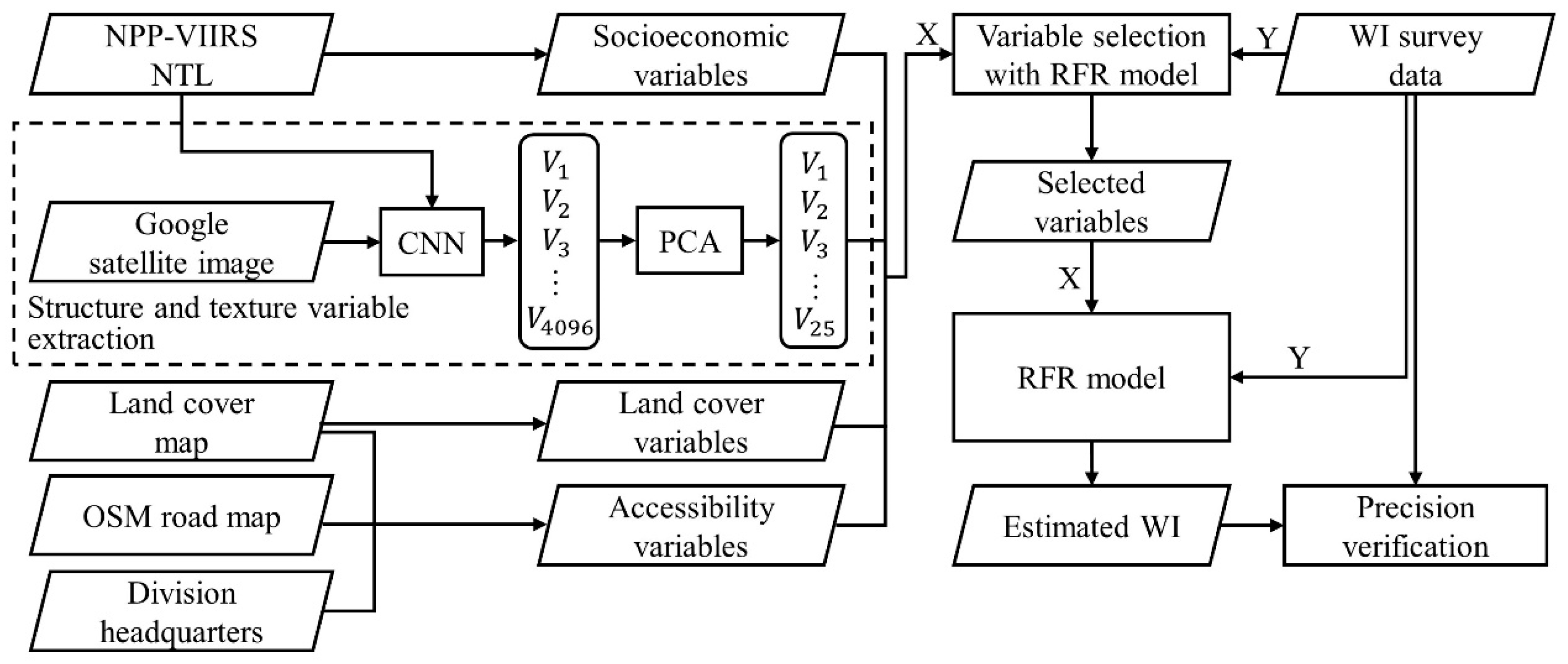
39]. In this study, we propose a RFR model to estimate poverty at 10-km resolution by integrating multi-source datasets, including NTL data, Google satellite imagery, land cover data, road data and division headquarter location data. The remainder of the article is organized as follows.
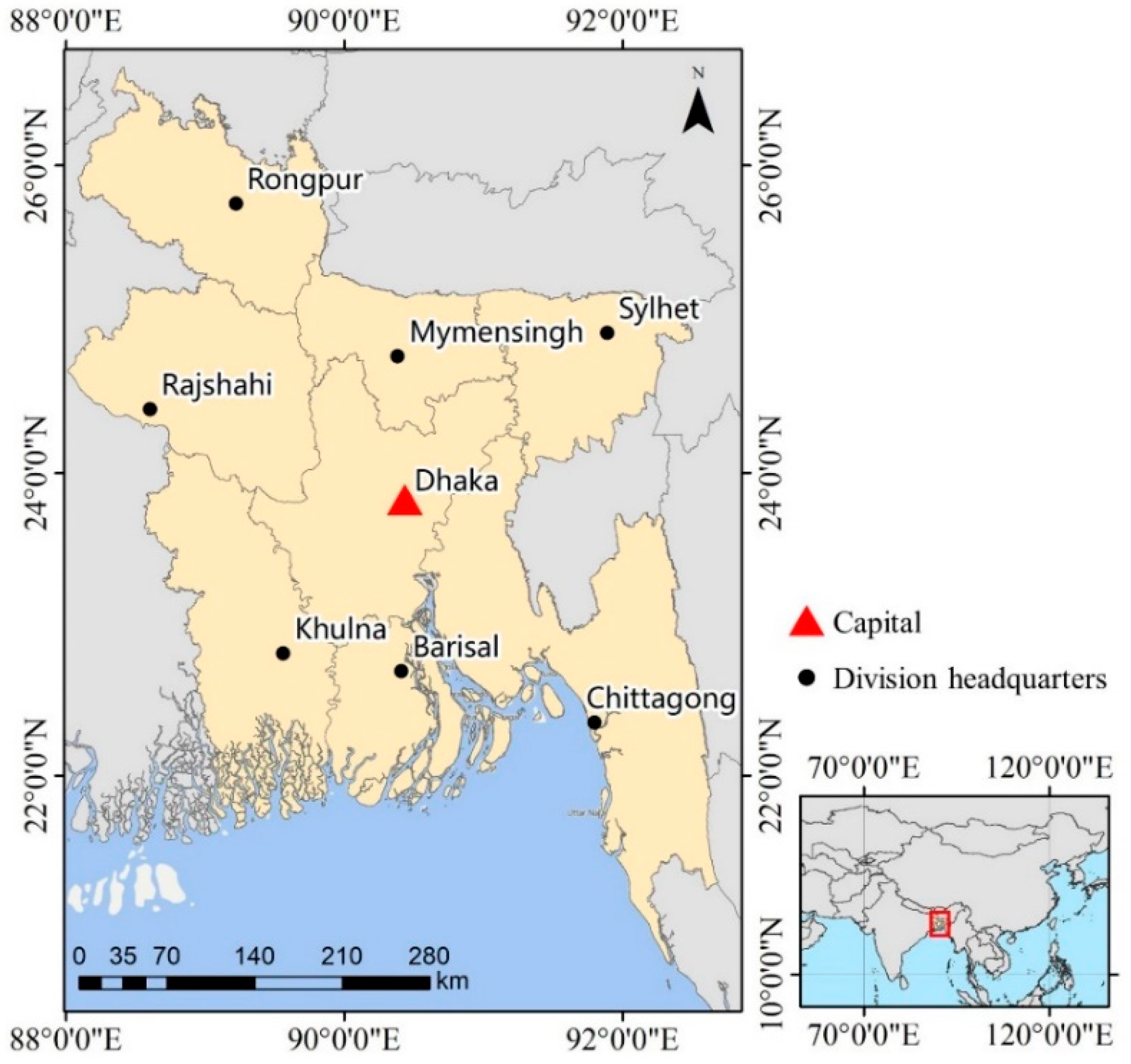
Section 2 introduces the study area, data and methods used in this study.
Section 3 and
Section 4 present the results and discussion, respectively. Conclusions are summarized in
Section 5.
4. Discussion
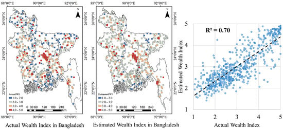
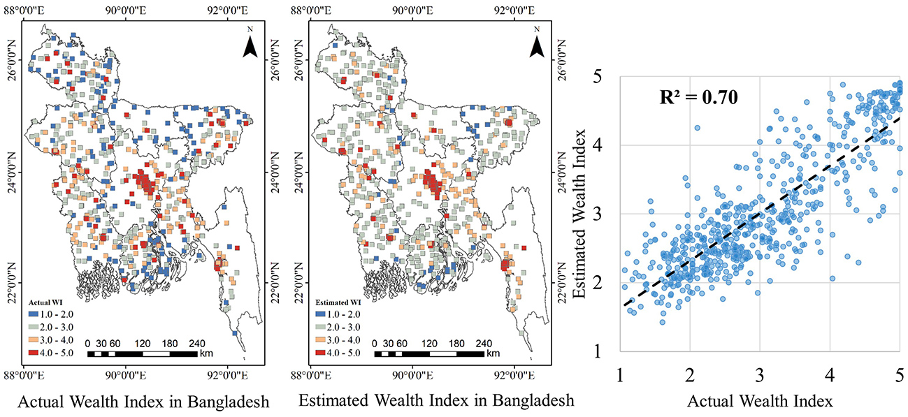
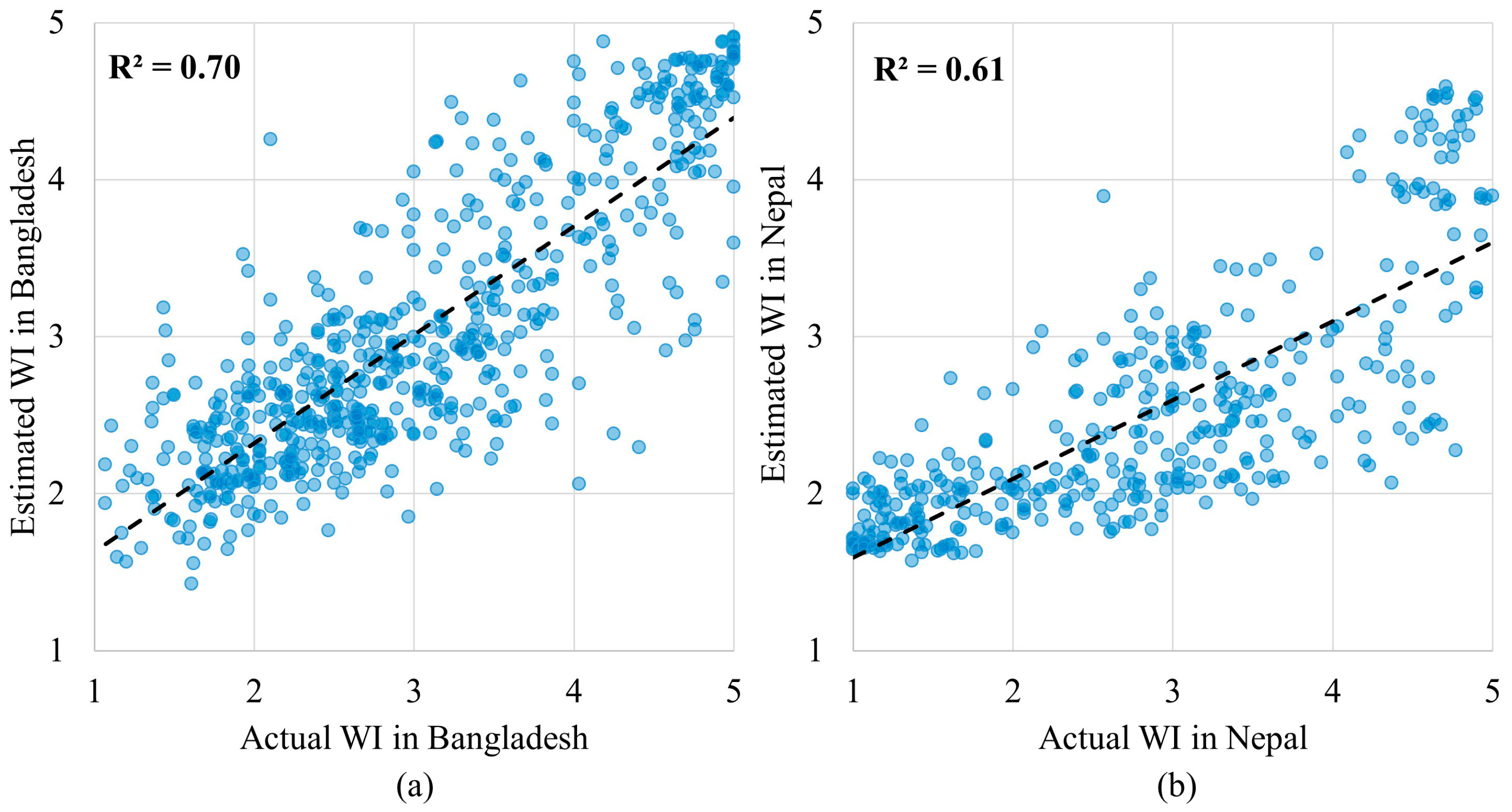
This study applies a RFR model for estimating poverty at 10 km × 10 km spatial resolution using variables extracted from multiple data sources in Bangladesh. The R
2 between the estimated WI from 10-fold cross validation and the actual WI in Bangladesh is 0.70, which is relatively high compared to the results in previous research [
23,
25,
27,
28]. By applying the model trained in Bangladesh to Nepal, we tested the replicability of the model in different geographical context. The R
2 between the estimated and actual WI of 0.61 in Nepal indicated a relatively good generalization ability compared to the previous research [
28], which used a model trained in one country to estimate WI in other five countries with R
2 between estimated and actual WI ranging from 0.24 to 0.71. Our results show that a relatively accurate estimation can be made by using multiple environmental data sources. Therefore, for countries that lack survey data, the RFR model can be used by using training data in other countries to estimate poverty.
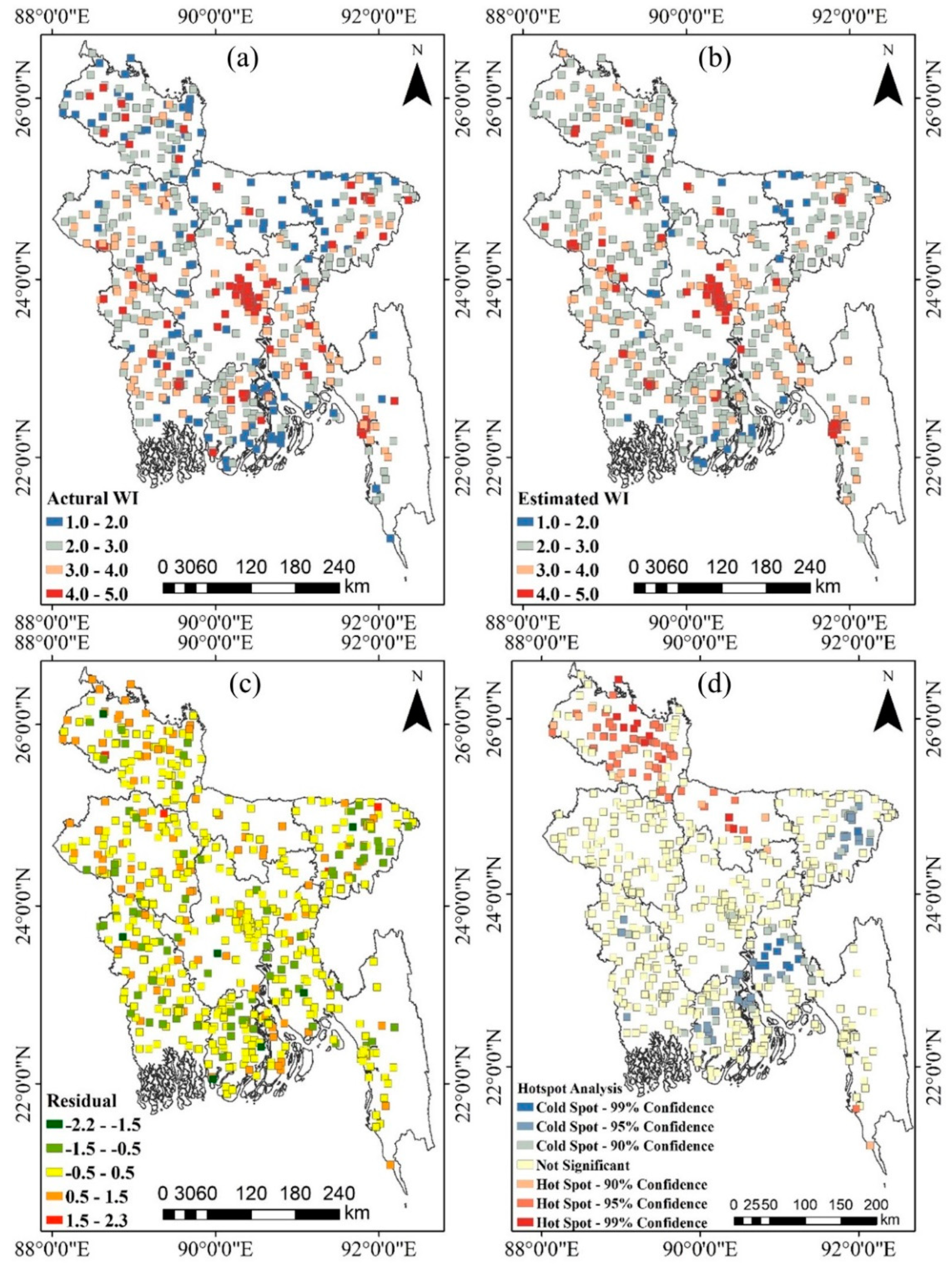
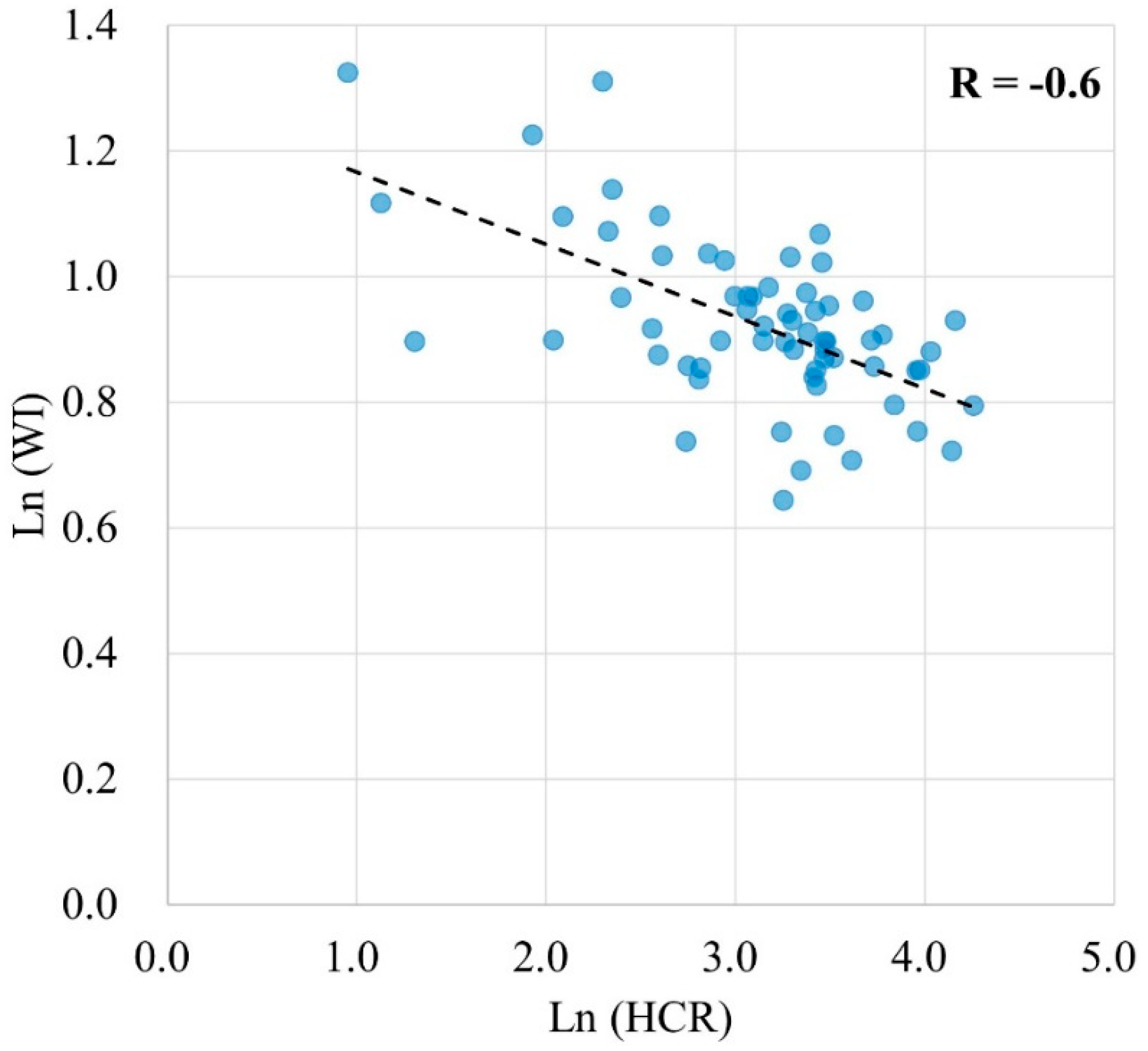
The overall small residuals indicate a relatively accurate predictive power of our model. However, the results of the residual analysis also indicate that the proposed RFR model tends to underestimate high WI values and overestimate low WI values. That is because the final result of a RFR model is the average result over all the trees that formed the RFR. Therefore, it is impossible to predict either beyond the range of response values in the training data, or within the entire range of the response values [
65]. That would result in the underestimation of high values and overestimation of low values. This is an inherent limitation of the RFR model. When we aggregate the data to the district-level, and valid the model results with the HCR data, a negative correlation between the average WI and the poverty HCR was established, which is in line with our perception that poor areas tend to have lower average household assets and a higher proportion of poor people. The correlation between them was not very high (r = −0.60) due to the different measuring methods. WI was calculated based on household’s ownership of several assets as a reflection of wealth, whereas poverty HCR was computed as the proportion of poor people in each division. Despite this difference, it still shows that the aggregated WI can partially reflect the district-level poverty HCR.
To test whether our RFR model improves upon the direct use of Google satellite images or NTL to estimate WI, we compared the results from our RFR model with the outcome from two other models. The first was a transfer learning model that used the 4096-dimensional feature vector from the Google satellite images along with the WI data to train a ridge regression model to estimate the WI [
28]. The second model used a linear regression to estimate the WI from the log-transformed NTL data [
65]. We also compared our results with a RFR model that excludes variables extracted from Google satellite images. This comparison was practiced to assess the extent the model without Google satellite images can estimate WI given that time-consuming nature for computing the Google image data.
Table 5 shows the R
2 between the estimated and actual WI from all four methods.
The R
2 of the linear regression model using the log-transformed NTL was 0.58, which was lower than the R
2 of our proposed RFR model. The R
2 of the transfer learning model was 0.63. Previous research [
28] using the same method got the R
2 values of 0.55, 0.58, 0.66, 0.69, and 0.75 for five countries in Africa. Our result was within this range, indicating that the transfer learning model can be applied to Bangladesh and our estimation was reasonable. Compared to models that used NTL and Google satellite imagery in isolation to estimate poverty, our RFR model had a higher accuracy. This proves that our RFR model can increase the poverty estimation accuracy by adding different types of data. The R
2 of the RFR model that excludes features extracted from Google satellite images was 0.66, which was slightly lower than the proposed RFR model and higher than the transfer learning model that used Google satellite images only. Considering the time-consuming nature of computing the Google image data, the RFR-based model without using Google satellite images was more efficient and accurate than the transfer learning model.
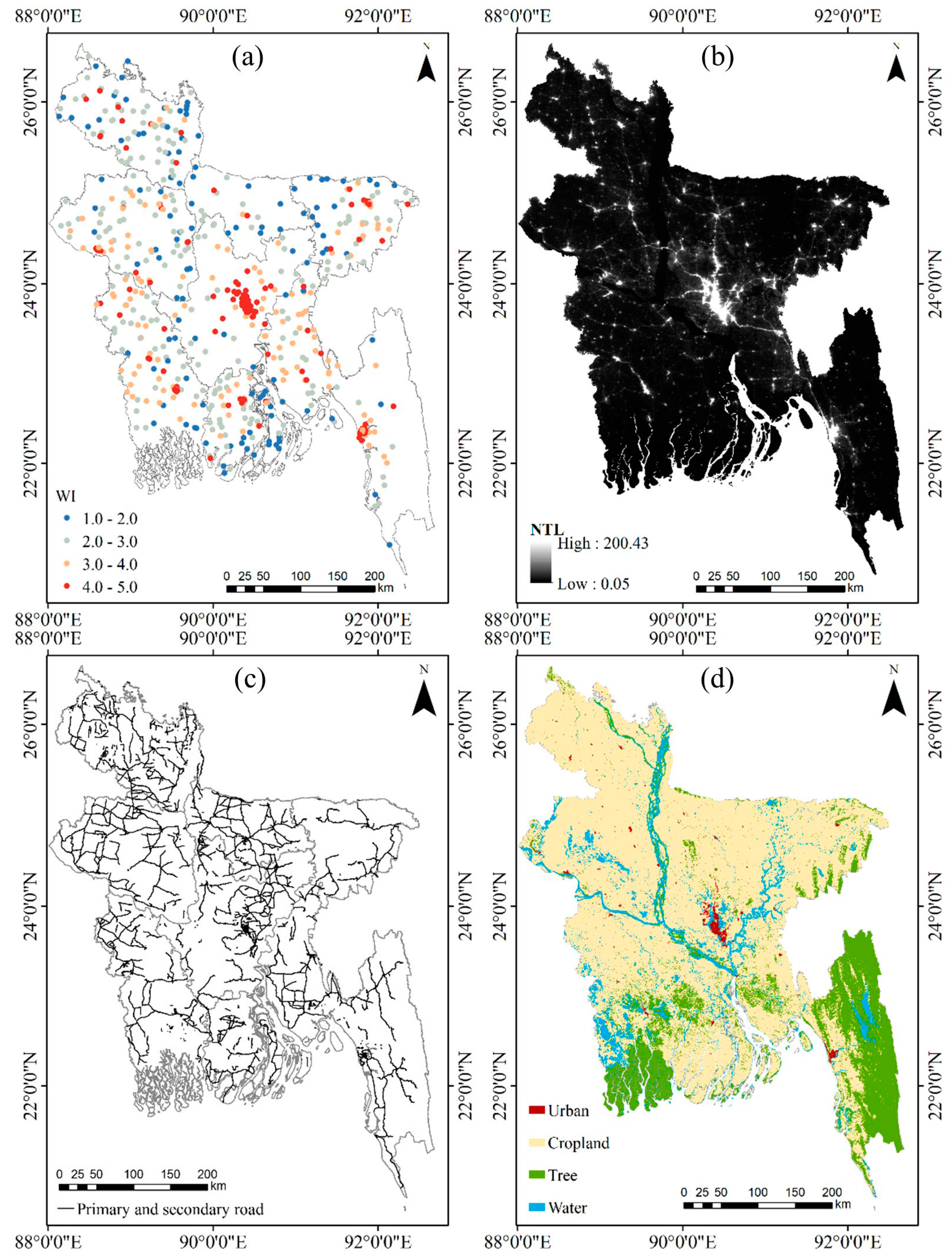
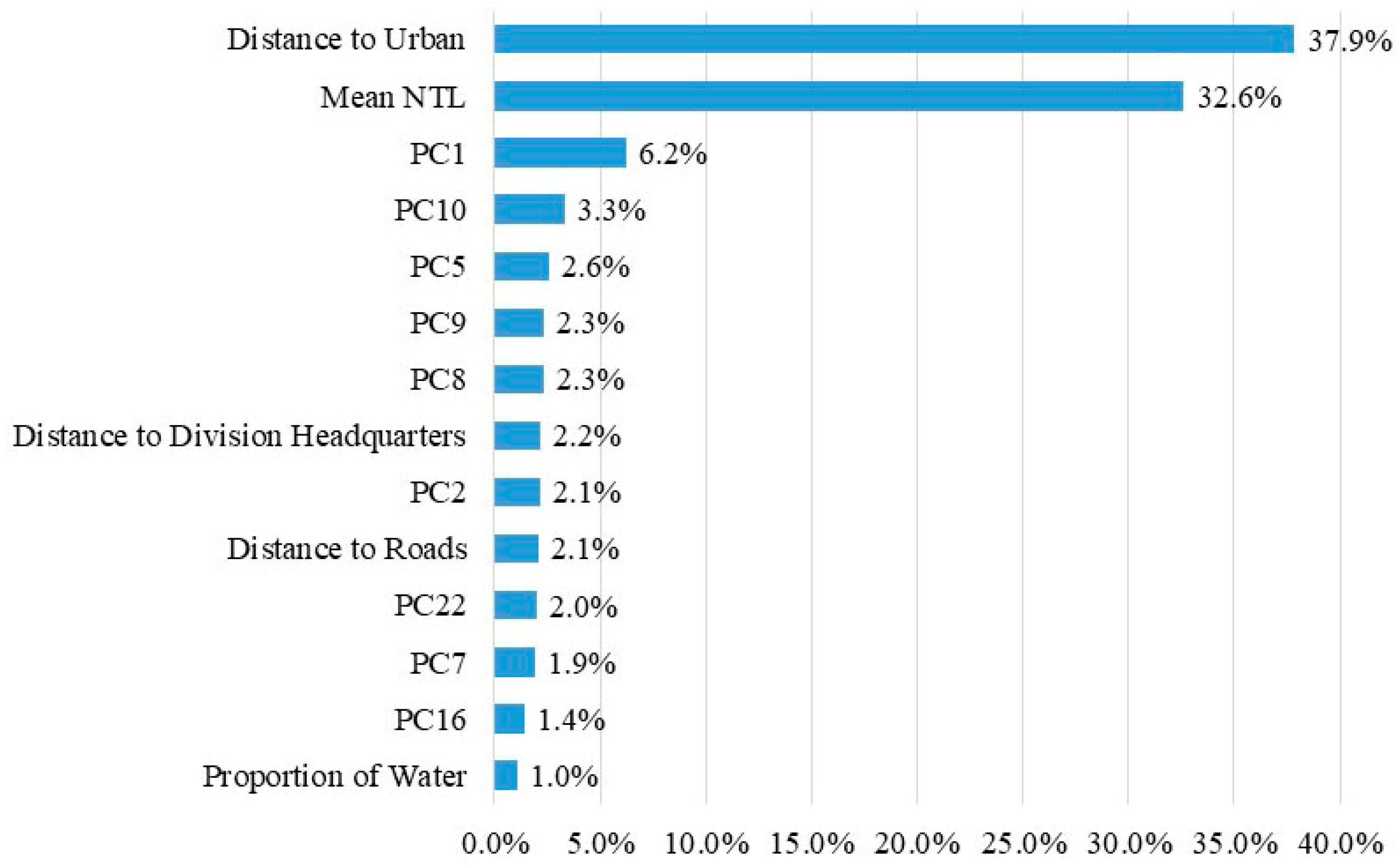
The analysis of the variables’ importance shows that accessibility variables were the most import variables to estimate poverty, indicating that the variations in distance to roads, urban and division headquarters are most likely to lead to variations in poverty level. This also illustrates that communities in regions that are far from roads, urban and large cities tend to have limited resources and are therefore more inclined to poverty. Socioeconomic variables can directly reflect the economic condition and were assessed to be the second important variables. Amongst the three socioeconomic variables, minimum NTL and maximum NTL radiance were discarded because their variations can be expressed by the variation of the mean NTL. Amongst the land cover variables, the proportion of urban, cropland, and tree were discarded probably because the features extracted from Google satellite images can reflect more detailed land cover information by providing the spatial distribution of each type of land cover rather than the proportion.
The collinearity analysis of the variables shows that there is strong collinearity between PC1 and mean NTL. Besides, the correlation between some other variables, although not strong, was statistically significant. Despite this, the RFR model still has good ability to estimate poverty. The analysis of the importance of variables shows that all of these variables contribute to the RFR model. In addition, discarding either of them would result in a decrease in accuracy of the model, indicating that the differences between them still contribute to the RFR model. This shows that RFR model has the ability to handle multicollinearity because the variables used to train each tree in a RFR model are different given that each of them were selected randomly from all variables. Therefore, the RFR model is not constrained to selecting only independent variables to estimate poverty.
5. Conclusions
There is pressing need to identify reliable data for poverty estimation in the absence of poverty survey data. While remote sensing data and road maps can reflect some of the environmental characteristics that are associated with poverty, existing studies are limited in using such data in isolation rather than collectively to represent the multidimensional construct of poverty and improve the accuracy of estimation. This study explores an integration of multi-source data and a RFR model to estimate poverty at 10 km × 10 km resolution. The WI for household clusters was used as the dependent variable to reflect poverty level and model training was conducted in Bangladesh. Thirty-six independent variables representing four poverty dimensions including socioeconomic status, structure and texture, land cover, and accessibility were extracted from NPP-VIIRS NTL data, Google satellite imagery, land cover map, OSM road map, and the division headquarter map. Following a vigorous variable selection procedure, 14 variables that offered the best predictive ability of the RFR model were reserved to train the final RFR model. After training the RFR model, we verified the accuracy of the model in three ways. Firstly, we calculated the R
2 between the actual WI and the WI estimated from 10-fold cross validation in Bangladesh. A high overall accuracy of our RFR model with an R
2 of 0.70 was obtained to estimate poverty at 10 km × 10 km resolution. Analysis of the residuals shows that the RFR model tends to underestimate the high WI values and overestimate the low WI values. Secondly, the trained RFR model was applied to Nepal to test whether the model trained in one country can be used to estimate poverty in another country. The R
2 between the actual and estimated WI in Nepal was 0.61, indicating a good generalization ability of our model. Thirdly, we calculated the average WI of each district and compared it to the district level poverty HCR. The r of −0.60 showed a relatively strong negative correlation between them, indicating that the results of our RFR model can reflect poverty HCR at the district level to some extent. Gini importance was used to assess the explanatory power of each variable. Accessibility variables were the most important variables to estimate WI with the total importance of 42.2%, followed by socioeconomic variables (32.6%), structure and texture variables (24.1%), and land cover variables (1.0%). Although there was multicollinearity between variables, the proposed RFR had good ability to estimate poverty, which confirmed the finding that the RFR model has the ability to handle multicollinearity [
35,
38]. Compared to other methods that used NTL or Google satellite imagery in isolation to estimate poverty, our method has produced higher accuracy by using multi-source data. All data we use in this study, including NPP-VIIRS NTL data, Google satellite imagery, land cover data, OSM road map, and division headquarter location map, are publicly and globally available. Therefore, the proposed model can be easily applied to other countries or regions.
This study has some limitations. Firstly, the acquisition time of the data in use was different. The WI survey data were obtained in 2014, while the NTL and land cover data were obtained in 2015, the road map was in 2018 and Google satellite data were from 2015 to 2017. As the Bangladesh government has been working to eradicate poverty, the poverty level could be changing every year. Therefore, differences in data acquisition time could result in reduced estimation accuracy. Secondly, the location of the WI data was not accurate due to the up to 5 km of positional errors added by the data collection agencies to protect the privacy of survey respondents, which could also contribute to noise in the model accuracy assessment. Furthermore, given the 5-km positional error, we estimated WI at 10-km resolution, which was relatively rough. Further training and validation of the estimation can be achieved and higher resolution estimation can be conducted as more environmental data and more accurate poverty survey data become available.

 ,
, 


