Testing Accuracy of Land Cover Classification Algorithms in the Qilian Mountains Based on GEE Cloud Platform

Abstract

The Qilian Mountains (QLM) are an important ecological barrier in western China. High-precision land cover data products are the basic data for accurately detecting and evaluating the ecological service functions of the QLM. In order to study the land cover in the QLM and performance of different remote sensing classification algorithms for land cover map** based on the Google Earth Engine (GEE) cloud platform, the higher spatial resolution remote sensing images of Sentinel-1 and Sentinel-2; digital elevation data; and three remote sensing classification algorithms, including the support vector machine (SVM), the classification regression tree (CART), and the random forest (RF) algorithms, were used to perform supervised classification of Sentinel-2 images of the QLM. Furthermore, the results obtained from the classification process were compared and analyzed by using different remote sensing classification algorithms and feature-variable combinations. The results indicated that: (1) the accuracy of the classification results acquired by using different remote sensing classification algorithms were different, and the RF had the highest classification accuracy, followed by the CART and the SVM; (2) the different feature variable combinations had different effects on the overall accuracy (OA) of the classification results and the performance of the identification and classification of the different land cover types; and (3) compared with the existing land cover products for the QLM, the land cover maps obtained in this study had a higher spatial resolution and overall accuracy.

1. Introduction

Due to a combined influence of natural processes and human activities, the global land cover is changing rapidly [1]. With the advancement in multisource remote sensing data, land cover and its changes have been closely studied in recent years [2]. Accurate and reliable land cover data is indispensable, as it provides basic information related to scientific research in areas such as agricultural, environmental protection, and global change [3,4,5,6]. However, accurate land cover map** and its changes are still facing many challenges due to land surface heterogeneity and spectral confusion, especially in higher-resolution map**.

Since the late 1990s, many land cover data products with different resolutions have been developed, including the University of Maryland (UMD) classification [7], the International Global Biosphere Programme (IGBP) DISCover [8], Global Land Cover 2000 (GLC2000) [9], MCD12Q1 [10], GlobCover [11], and the Climate Change Initiative-Land Cover (CCI-LC) [12]; however, the resolution of these land cover products are low, ranging from 300 m to 1 km. Copernicus Global Land Service-Land Cover 100 (CGLS-LC100) delivers a global land cover map at 100 m spatial resolution. Since 2015, three collections of CGLS-LC100 have been released [13]. CORINE Land Cover (CLC) is a standard dataset for land cover in Europe. There are now five versions, including CLC-1990, CLC-2000, CLC-2006, CLC-2012, and CLC-2018. The quality and accuracy of datasets have been greatly improved [14]. The Google Earth Engine (GEE) is a global geospatial analysis platform that was developed based on cloud technology [15]. Due to its powerful computing functions and the advantages of online data calculations and visual analysis, it has a wide range of applications in land cover map** research. Based on the high spatial and temporal resolution of the remote sensing data provided by the GEE, different high-resolution land cover data products have been developed. The representative land cover products on a global scale include the following. Chen et al. used a Landsat time series and HJ-1 satellite remote sensing images to produce a global land cover product (GlobeLand30) with a spatial resolution of 30 m [16]. Gong et al. used Landsat TM/ETM+ data and Sentinel-2 data, respectively, for the fine resolution (30 m) observation and monitoring of the global land cover (FROM-GLC30) [17] and the fine resolution (10 m) observation and monitoring of the global land cover (FROM-GLC10) [18] based on the GEE platform. Zhang et al. produced two global land cover products with high spatial resolutions; i.e., the Global Land Cover with Fine Classification System in 2015 (GLC_FCS30-2015) and the Global Land Cover with Fine Classification System in 2020 (GLC_FCS30-2020) [19,20]. Gao et al. used the open validation dataset (LUCAS) to evaluate the performance of the GLC_FCS30-2015 and compared it with the GlobeLand30-2010 and FROM_GLC-2015 [21]. Among the land cover products listed above, MCD12Q1, GlobCover, CGLC-LC100 collection 3, and CORINE Land Cover are available in GEE.

Although there are a variety of widely used land cover products, such as those mentioned above, due to the differences in the data sources, classification schemes, and classification methods of the different data products, their adaptability and accuracy in some specific areas tend to be uncertain. Therefore, it is vital to produce more precise and accurate land cover products for a certain area. For example, Zhang et al. used the Sentinel-2 time series based on the tile model and the RF algorithm based on the GEE platform to automatically generate a high-resolution land cover map of Madagascar, with a high overall accuracy (OA) of 89.2% [22]. Zeng et al. used Landsat 8 image data and the RF algorithm based on the GEE platform to analyze watershed land cover map** in Nzhele and Levhuvu, with an OA of 76.43% [23]. Midekisa et al. used the Landsat 7 ETM+ surface reflectance data in 2000 and 2015 and the RF algorithm based on the GEE platform to automatically generate the 30 m resolution cover map of the African continent and analyzed its change characteristics [24]. Based on Landsat 8 images, RF algorithm, and GEE platform, Tassi et al. produced the land cover map of Maiella National Park in Italy [25]. Despite all this research, the available studies still lack a comparison of the classification performances and effects of the different classifiers in the same research area.

The Qilian Mountains (QLM) are an important ecological security barrier in western China, and have strategic significance for the whole country. A high-resolution and accurate land cover map is a key dataset for ecosystem function monitoring, ecological protection, and restoration in this region. The current high-spatial-resolution global land cover products such as GlobeLand30 [16], FROM-GLC30 [17], and FROM-GLC10 [18] all include land cover maps of the QLM. In addition, China’s high-spatial-resolution land cover products, such as China’s Multiperiod Land Use Land Cover Remote Sensing Monitoring Dataset (CNLUCC) [26] and SPECLib-Based Land Cover [27], also include land cover maps of this region. On the regional scale, Yang et al. developed the Land Cover Dataset for the QLM Area from 1985 to 2019 (V2.0) based on the GEE platform using Landsat 8 data, with an OA of 92.19% [28]. Wang et al. used MODIS data, based on the GEE and combined with topographic features, to conduct land cover classification research on the QLM [29]. However, the existing land cover products have inconsistencies and uncertainties in the classification results of the QLM, lacking a performance comparison of the different remote sensing classification algorithms in the QLM. Therefore, it is necessary to use different remote sensing classification algorithms to study the QLM, produce more accurate high-resolution land cover products, and assess the performances of the different classification algorithms.

According to the research background presented above, and based on the GEE cloud platform, Sentinel-2 remote sensing images were used to produce the land cover classification products for the QLM, with a spatial resolution of 10 m. Specifically, the research content of this study is as follows: (1) to evaluate the performance of the GEE cloud platform in land cover research in the QLM; (2) to assess the performances and accuracies of the different remote sensing classification algorithms in the land cover classification of the QLM; (3) to analyze the impacts of different characteristic variable combinations on the classification results while participating in classification; and (4) to compare and analyze the classification results obtained in this study using existing land cover products.

2. Materials and Methods

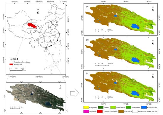
2.1. Study Area

The Qilian Mountains (35°48′–40°05′N, 93°18′–103°54′E) are located in northwestern China, to the northeast of the Qinghai-Tibetan Plateau (QTP), in Gansu and Qinghai Provinces (Figure 1). The total area is 1.84 × 10⁵ km², with an elevation of 1623–5766 m [30]. The QLM is an important ecological security barrier in western China. Many inland rivers that originate from the QLM are important freshwater sources for the Hexi Corridor, maintaining the freshwater balance and oasis stability in the area. The QLM are composed of a number of NW-trending high mountains and valleys. The overall terrain characteristic is that the west is higher than the east, with high altitudes and complex and special geomorphological features. The QLM have a typical continental plateau climate, which is dry and cold, and it gradually becomes colder and drier from east to west. The annual average temperature is low, about 0.6 °C; and the ranges of annual and daily temperature are relatively large. The annual precipitation is about 400–700 mm, and it decreases from east to west and increases with elevation. The region has a high solar radiation intensity, with most areas receiving more than 2800 h of sunshine. The land cover types in the QLM are diverse, mainly including croplands, forests, grasslands, shrublands, wetlands, water bodies, construction lands, and bare lands, among which the grasslands and meadows account for a large percentage of the total area. The main crops are wheat, oilseed rape, highland barley, oats, maize, broad beans, and potatoes.

2.2. Data Preparation

2.2.1. Sentinel-2 Image Data

The MultiSpectral Instrument (MSI) equipped on the Sentinel-2 satellite is a high-resolution multispectral imaging sensor. The Sentinel-2 mission comprises a constellation of two polar-orbiting satellites (2A and 2B). Sentinel-2 has an inter-resolution of 5d after the two satellites are networked, and carries a multispectral imager. The spatial resolution of the visible light bands and near-infrared band is 10 m [31]. The remote sensing data used in this study were the Sentinel-2 Level-2A products for the 2020 and 2021 plant growth season (from the beginning of June to the end of August). A total of 899 Sentinel-2 images were selected in QLM, and each image included 12 spectral bands and 3 quality assessment (QA) bands. The data acquisition and preprocessing were conducted through online code writing on the GEE cloud platform. The QA60 band of the images was used and set as a cloud mask to remove the clouds from the images in order to obtain a cloud-free image.

2.2.2. Sentinel-1 Image Data

The Sentinel-1 data are C-band synthetic aperture radar (SAR) data [32]. Sentinel-1 images provided by the GEE cloud platform have undergone preprocessing procedures such as thermal noise removal, radiation calibration, and terrain correction. A total of 398 Sentinel-1 images that were synchronized with Sentinel-2 data were used in this study, and the data acquisition and processing were conducted using the GEE platform.

2.2.3. SRTM Data

The Shuttle Radar Topography Mission (SRTM) data were jointly measured by the National Aeronautics and Space Administration (NASA) and the National Imagery and Map** Agency (NIMA) [33]. The product name of the digital elevation data provided in the GEE cloud platform was SRTMGL1_003, and the data acquisition and processing were conducted using the GEE platform.

2.2.4. Land Cover Datasets

The GlobeLand30 is a global land cover product produced by the National Geomatics Center of China [16]. The FROM-GLC30 is the first global 30 m spatial resolution land cover product, produced by Tsinghua University in 2013 based on Landsat images [17]. The FROM-GLC10 data were the latest results for the 2017 land cover produced by Tsinghua University, which used Sentinel-2 images and previous training samples based on Landsat data [18]. The Qilian Mountains 30 m land cover classification product data set (1985–2019) V2.0 (LCD-QLM (V2.0)) was also used in this study as auxiliary reference data [28]. The data were downloaded from the National Qinghai-Tibetan Plateau Science Data Center (http://data.tpdc.ac.cn, accessed on 24 September 2021). The basic information about the land cover products is presented in

Table 1. Basic information of existing land cover products.

Products	Data Source	Time	Spatial Resolution	Classification Algorithms
FROM-GLC30	Landsat TM/ETM+	2010, 2015, 2017	30 m	SVM, supervised classification
GlobeLand30	Landsat TM/ETM+, HJ-1	2000, 2010	30 m	Pixel-object-knowledge-based (POK-based) method
FROM-GLC10	Sentinel-2	2017	10 m	RF, supervised classification
Land Cover Dataset at Qilian Mountain Area from 1985 to 2019 (V2.0)	Landsat 8 TM/ETM+/OLI	1985, 1990, 1995, 2000, 2005, 2010, 2015, 2016, 2017, 2018, 2019	30 m	Supervised classification

.

2.3. Methods

Based on the GEE cloud platform and the remote sensing classification algorithms and remote sensing data it provided, this research aimed to classify the land cover in the Qilian Mountains. The research methods included the collection and optimization of the sample data, the construction of the feature space, and the machine learning classification algorithms and evaluation of classification results. The data processing and analysis flow diagram of this research is shown in Figure 2.

2.3.1. Sampling Strategies

The collection of accurate training and validation samples is a necessary condition for accurate land cover classification [34]. Unrepresentative and/or inadequate samples will result in significant uncertainty of the land cover classification results [35]. Taking into account the actual situation in the QLM and referring to the existing land cover classification system and products, the classification system of this study is shown in

Table 2. Land cover classification system.

Code	Class	Abbreviation	Description
1	Cropland	CO	A land cover type that is greatly affected by intensive human activities. It varies greatly from bare field to seeding to crop growing to harvesting in the course of a year. It includes paddy fields, greenhouse farming, and other arable and tillage land.
2	Forest	FO	Areas in which the tree cover percentage is >15% and the tree height is > 3 m, including natural forests, plantations, and fruit trees.
3	Grassland	GL	Areas in which the herbaceous cover percentage is >15%, including natural grassland and pastures.
4	Shrublands	SL	Area in which the shrublands’ height range is 0.3–5 m, and cover percentage is >15%, have unique texture.
5	Wetlands	WL	Usually has obvious high reflectivity in the NIR band; marshland covered with aquatic herbaceous plants; mudflats are also included.
6	Water bodies	WB	All inland waterbodies; dominated by natural waterbodies and artificial waterbodies.
7	Construction land	CL	Includes urban areas, rural areas, and industrial and mining land greatly affected by human activities.
8	Bare land	BL	Areas without vegetation cover, including wasteland, deserts, and the Gobi Desert.
9	Permanent snow and ice	PSI	Perennial snow and ice distributed in the high mountains.

. The classification system used in this study was the land cover classification system based on ecosystem types, and was divided into 9 categories: croplands (CO), forests (FO), grasslands (GL), shrublands (SL), wetlands (WL), water bodies (WB), construction land (CL), bare land (BL), and permanent snow and ice (PSI). The high-resolution satellite imagery of the Google Earth Engine was used as a base map; the sample points were selected from the areas where land cover changes have not occurred for many years, and the areas that were relatively uniform and had little interference from human activities to ensure the accuracy and authenticity of the sample data. Furthermore, the collected sample data were compared and verified with the 10 m ecosystem-type data of the Qilian Mountain Nature Reserve (part of the Qilian Mountains), which was obtained by artificial interpretation and field verification. The unit of each sample point was a pixel.

The quality and quantity control of sample point data was realized by the method of area estimation adjustment error [36,37,38,39]. In this way, the deviation caused by stratified sampling could be adjusted. Using sample data, the confusion matrix n_ij of the classification result could be calculated. A more informative presentation of the error matrix is the unbiased estimation p_ij of the area ratio in the unit i and j of the error matrix:

$$p_{ij}=W_i\frac{n_{ij}}{n_i}$$

(1a)

where W_i is the area ratio of land cover types to the total area of the study area in the classification results, and the proportion of the area classified as type i is:

$$W_i=\frac{A_i}{A_{tot}}$$

(1b)

where A_tot is the total area of the map, and A_i is the mapped area of land cover type i.

An unbiased estimator of the total area of type j is then:

$$A_j=A_{tot}\times p_j$$

(2a)

where p_j can be calculated using the following formula:

$$p_j={\displaystyle \sum }_i{W}_i\frac{n_{ij}}{n_i}$$

(2b)

The estimated standard error of the estimated area proportion is:

$$S\left(p_j\right)=\sqrt{{\displaystyle \sum }_{i=1}^q{W}_i^2\frac{\frac{n_{ij}}{n_i}\left(1-\frac{n_{ij}}{n_i}\right)}{n_i-1}}$$

(3)

The standard error of the error-adjusted estimated area is:

$$S\left(A_j\right)=A_{tot}\times S\left(p_j\right)$$

(4)

An approximate 95% confidence interval for A_j is:

$$A_j\pm 2\times S\left(A_j\right)$$

(5)

where the range of error is defined as the z-score multiplied by the standard error, and the value of the z-score is related to the confidence level (for 95% confidence, z = 1.96). When the area of each land cover types in the classification results was within the estimated area ranges, it could be considered that the sample data on which the classification results were based were reasonable. The method accurately quantified the classification error caused by inaccurate sampling, and the final number of sample points is shown in

Table A1. The number of sample points.

Code	Land Cover Types	Number
1	Croplands	328
2	Forests	1192
3	Grasslands	9103
4	Shrublands	113
5	Wetlands	199
6	Water bodies	703
7	Construction lands	261
8	Bare lands	8730
9	Permanent snow and ice	482
Total		21,111

(Appendix A). Using the ‘randomColumn’ function in the GEE cloud platform, 70% of the sample data could be randomly selected for the classifiers training and image classification, and 30% of the sample data were used for the verification and evaluation of classification results.

2.3.2. Feature Construct

• Spectral indices

Existing studies have shown that the application of remote sensing spectral indices can effectively improve the accuracy of the identification of different land cover types. In this study, the normalized difference vegetation index (NDVI) [40], the enhanced vegetation index (EVI) [41], the land surface water index (LSWI) [42], the normalized difference water index (NDWI) [43], the soil adjusted vegetation index (SAVI) [44], and the bare soil index (BSI) [45] were calculated using the GEE cloud platform based on the formulas for each spectral index, and each index was added to the original remote sensing image in turn (as shown in Figure 2). The calculation formulas for each index are as follows:

$$\mathrm{NDVI}=\frac{{\mathsf{\rho }}_{\mathrm{NIR}}-{\mathsf{\rho }}_{\mathrm{RED}}}{{\mathsf{\rho }}_{\mathrm{NIR}}{+\mathsf{\rho }}_{\mathrm{RED}}}$$

(6)

$$\mathrm{EVI}=2.5\times \frac{{\mathsf{\rho }}_{\mathrm{NIR}}-{\mathsf{\rho }}_{\mathrm{RED}}}{{\mathsf{\rho }}_{\mathrm{NIR}}{+6\times \mathsf{\rho }}_{\mathrm{RED}}-7{.5\times \mathsf{\rho }}_{\mathrm{BLUE}}+1}$$

(7)

$$\mathrm{LSWI}=\frac{{\mathsf{\rho }}_{\mathrm{NIR}}-{\mathsf{\rho }}_{\mathrm{SWIR}}}{{\mathsf{\rho }}_{\mathrm{NIR}}{+\mathsf{\rho }}_{\mathrm{SWIR}}}$$

(8)

$$\mathrm{NDWI}=\frac{{\mathsf{\rho }}_{\mathrm{GREEN}}-{\mathsf{\rho }}_{\mathrm{NIR}}}{{\mathsf{\rho }}_{\mathrm{GREEN}}{+\mathsf{\rho }}_{\mathrm{NIR}}}$$

(9)

$$\mathrm{SAVI}=\frac{{(\mathsf{\rho }}_{\mathrm{NIR}}-{\mathsf{\rho }}_{\mathrm{RED}}\left)\right(1+\mathrm{L})}{{(\mathsf{\rho }}_{\mathrm{NIR}}{+\mathsf{\rho }}_{\mathrm{RED}}+\mathrm{L})}$$

(10)

$$\mathrm{BSI}=\frac{\left({\mathsf{\rho }}_{\mathrm{RED}}{+\mathsf{\rho }}_{\mathrm{SWIR}}\right)-\left({\mathsf{\rho }}_{\mathrm{NIR}}{+\mathsf{\rho }}_{\mathrm{BLUE}}\right)}{\left({\mathsf{\rho }}_{\mathrm{RED}}{+\mathsf{\rho }}_{\mathrm{SWIR}}\right)+\left({\mathsf{\rho }}_{\mathrm{NIR}}{+\mathsf{\rho }}_{\mathrm{BLUE}}\right)}$$

(11)

where ρ_SWIR, ρ_NIR, ρ_RED, ρ_GREEN, and ρ_BLUE are the surface reflectance values of the shortwave infrared, near-infrared, red, green, and blue bands, respectively. L is the soil regulation factor, which ranges from 0 to 1 and is usually assigned a value of 0.5 to better reduce the background difference of the soil and eliminate the noise impact of the soil [44].

• Texture features

The texture features are an important attribute of remote sensing images, and different land cover types have different texture features. Based on the texture features, the accuracy of the recognition and classification can be improved [46]. The Gray-Level Co-occurrence Matrix (GLCM) is a classic method to extract the texture features [47]. It extracts textures through the conditional probability density between gray levels of remote sensing images, and is diffusely used in land cover classification research. The calculation of the GLCM can be obtained through the “glcmTexture” function in the GEE cloud platform. In this study, several commonly used texture features were selected for use in the classification, including the feature parameters of angular second moment (asm), contrast (con), correlation (corr), variance (var), inverse different moment (idm), sum average (savg), and entropy (ent) based on NDVI. The calculation of each feature variable was based on GLCM, they were dimensionless, and their range of values was not completely uniform.

• Radar features

Studies have shown that SAR data are sensitive to land cover types such as water bodies, construction lands, and croplands [23]. The radar variables involved in the construction of the feature variables in this study included the backscatter coefficients of the Sentinel-1 data in VV polarization and VH polarization modes.

• Terrain features

In the recognition and classification of remote sensing images, the participation of terrain features can improve the accuracy of the classification. Therefore, based on the SRTMGL1_003 digital elevation data product, the “ee.Terrain.products” function provided by GEE was used to calculate the aspect, hill shade, slope, and elevation, and they were added to the remote sensing images as independent features.

According to the feature variables described above, the classifications of image were conducted in five feature variable combinations. In the first input feature variable combination, only spectral bands of Sentinel-2 participated in the classification of the image, and then the feature variable combinations of spectral indices, terrain features, radar features, and texture features were added in turn.

2.3.3. Classification Algorithms

At present, remote sensing classification methods such as the support vector machine (SVM), the classification regression trees (CART), and the random forest (RF) algorithms have been widely used in land cover map** and crop type identification [4]. In order to analyze the differences in the accuracies of the extraction and classification of the different land cover types when using different classification algorithms, and when using the same feature variable combination and the differences in the accuracies of the extraction and classification of different land cover types when using the same classification algorithm but different combinations of feature variables, three classification algorithms were used in this study. These three classification algorithms are introduced below.

• Support Vector Machine

The support vector machine (SVM) was proposed by Vapnik in 1995 [48]. The SVM has significant advantages in terms of nonlinear problems, small samples, and a high dimensionality. It is widely used due to its small training samples and support for high-dimensional feature spaces. The parameters that need to be adjusted when using the SVM to classify remote sensing images are the kernel function type, the gamma value of the kernel function, and the cost parameter.

• Classification and Regression Tree

The classification and regression tree (CART) was proposed by Breiman et al. in 1984 [48]. It is widely used in land cover extraction and remote sensing image classification research due to its simple structure, fast calculation speed, and the advantage of being easy to understand. The parameters that need to be optimized when using CART to classify remote sensing images are the maximum and minimum numbers of leaf nodes in each tree.

• Random Forest

The random forest (RF) algorithm was proposed by Leo Beriman in 2001 [49]. Studies have shown that the RF has the advantages of stability, rapidity, and high precision in processing remote sensing data; and therefore, it has become the most widely used classifier among current remote sensing classification algorithms. It has important applications in crop extraction, image classification, and agricultural regression models [50,51]. The two main parameters that need to be adjusted and optimized for the RF when classifying remote sensing images are the number of decision trees that need to be created and the minimum number of leaf nodes. Studies have indicated that the values of the RF parameters have little effect on the accuracy [51], so the number of decision trees was set as 300. Additionally, when using RF for classification in GEE, the importance score of the parameters participating in the classifier can be calculated by using the “explain” function. The value of the importance score is not absolute, and there is no uniform and fixed value range, but changes with the number of sampling data and feature parameters participating in the classification [52,53]. The importance and contribution of the feature parameters participating in the classification can be determined by the relative value of the importance score in a specific situation.

2.3.4. Accuracy Assessment

The confusion matrix is a method that is commonly used to assess the accuracy of image classifications [54]. In this study, the calculation of the confusion matrix was conducted through online programming of the GEE cloud platform, and then the overall accuracy (OA), Kappa coefficient, producer accuracy (PA), and user accuracy (UA) were calculated. Among them, the OA and the Kappa coefficient could fully reflect the comprehensive accuracy of the results, and the PA and UA could be used to assess the classification accuracy of a specific land cover type. The calculation formulas were as follows:

$$\mathrm{OA}=\frac{{{\displaystyle \sum }}_{\mathrm{i}=1}^{\mathrm{n}}{\mathrm{X}}_{\mathrm{ii}}}{\mathrm{N}}\times 100\%$$

(12)

$$\mathrm{PA}=\frac{{\mathrm{X}}_{\mathrm{ii}}}{{\mathrm{X}}_{+\mathrm{i}}}\times 100\%$$

(13)

$$\mathrm{UA}=\frac{{\mathrm{X}}_{\mathrm{ii}}}{{\mathrm{X}}_{\mathrm{i}+}}\times 100\%$$

(14)

where N is the total number of samples used for the accuracy assessment; n is the total number of columns in the confusion matrix; ${\mathrm{X}}_{\mathrm{ii}}$ is the number of samples in the i-th row and i-th column in the confusion matrix; and ${\mathrm{X}}_{\mathrm{i}+}$ and ${\mathrm{X}}_{+\mathrm{i}}$ are the total number of samples in the i-th row and i-th column, respectively. The uncertainty analysis of the accuracy of classification results is realized by calculating the error range, which is defined as the z-score multiplied by the standard error [36].

In this study, all of the data processing and calculations, including data acquisition, data processing, composition of images, construction of feature space, calculation of parameters, implementation of classifiers, and calculations of confusion matrices, were all implemented by the GEE JavaScript API.

3. Results

3.1. Classification Results and Accuracy of Classification Results

Remote sensing classification algorithms, including SVM, CART, and RF, were used to classify the Sentinel-2 composite images in the QLM and to analyze the ability of the different classifiers to identify land cover types in high spatial resolution images. The land cover results based on the three classification algorithms are shown in Figure 3.

The results showed that the classification results obtained using the different remote sensing classification algorithms had high consistency in terms of the proportions and the distribution characteristics of the land cover types. Among them, bare land and grassland accounted for the largest proportion of the study area, accounting for more than 90%. The grassland was mainly distributed in the eastern and central regions of the QLM, and the relatively warm and humid valleys in the west were also distributed within a small area. The bare land was widely distributed in the western part of the QLM, where the temperature is low and the precipitation is scarce. In addition, the cropland was concentrated in the eastern basin, the middle reaches of the Datong River, and the plains on the northern slope of the northeastern part of the mountains, where the land is flatter, with abundant water resources and suitable temperatures. The forests were distributed in the valleys in the middle and eastern parts of the study area and on the northern slopes of the QLM in the northeast. The permanent snow and ice were distributed in the mountainous areas with higher elevations (4891 m on average) in the western and central parts of the study area.

The confusion matrix of the classification results obtained using the different remote sensing classification algorithms is shown in

Table 3. Confusion matrix of the classification results of the three remote sensing classification algorithms.

Methods	Land Cover Types	CR	FO	GL	SL	WL	WB	CL	BL	PSI	PA
SVM	CR	67	5	43	0	1	0	0	2	0	0.57 ± 0.09
	FO	2	319	45	0	0	0	0	0	0	0.87 ± 0.03
	GL	19	15	2669	0	0	0	0	19	0	0.98 ± 0.01
	SL	2	18	10	5	0	0	0	0	0	0.14 + 0.12
	WL	1	0	38	0	12	1	0	11	0	0.19 ± 0.10
	WB	1	0	0	0	1	214	2	11	0	0.93 ± 0.03
	CL	1	0	1	0	0	0	60	6	0	0.88 ± 0.08
	BL	0	1	18	0	0	0	5	2590	0	0.99 ± 0.01
	PSI	0	0	1	0	0	0	0	2	126	0.97 ± 0.03
	UA	0.72 ± 0.09	0.89 ± 0.03	0.94 ± 0.01	1.00 ± 0	0.86 ± 0.14	0.99 ± 0.01	0.90 ± 0.07	0.98 ± 0.01	1.00 ± 0
	OA	0.96 ± 0.01
	Kappa	0.93
CART	CR	66	0	35	0	4	1	0	1	0	0.62 ± 0.09
	FO	0	327	28	12	0	0	0	0	0	0.89 ± 0.03
	GL	43	29	2617	14	12	0	1	38	0	0.95 ± 0.01
	SL	0	10	5	21	0	0	0	0	0	0.58 ± 0.16
	WL	5	0	15	2	23	2	1	7	0	0.42 ± 0.13
	WB	0	0	0	0	1	190	1	3	0	0.97 ± 0.02
	CL	0	0	1	0	1	0	60	8	0	0.86 ± 0.08
	BL	2	0	30	0	7	6	8	2585	0	0.98 ± 0.01
	PSI	0	0	1	0	0	0	0	0	145	0.99 ± 0.01
	UA	0.57 ± 0.09	0.89 ± 0.03	0.96 ± 0.01	0.43 ± 0.14	0.48 ± 0.14	0.95 ± 0.03	0.85 ± 0.08	0.98 ± 0.01	1.00 ± 0
	OA	0.95 ± 0.02
	Kappa	0.93
RF	CR	78	0	24	0	8	1	0	2	0	0.69 ± 0.09
	FO	0	329	24	0	0	0	0	0	0	0.93 ± 0.03
	GL	13	7	2717	0	1	1	0	13	0	0.99 ± 0.01
	SL	0	7	5	17	0	0	0	0	0	0.59 ± 0.18
	WL	0	0	19	0	28	2	0	4	0	0.53 ± 0.13
	WB	0	0	0	0	1	190	1	1	3	0.97 ± 0.03
	CL	1	0	1	0	0	1	63	9	0	0.84 ± 0.08
	BL	0	0	10	0	0	0	0	2567	0	0.99 ± 0.01
	PSI	0	0	0	0	0	0	0	1	144	0.99 ± 0.01
	UA	0.85 ± 0.07	0.96 ± 0.02	0.97 ± 0.01	1.00 ± 0	0.74 ± 0.14	0.97 ± 0.02	0.98 ± 0.02	0.99 ± 0.01	0.98 ± 0.02
	OA	0.97 ± 0.01
	Kappa	0.96

CR = cropland; FO = forests; GL = grassland; SL = shrublands; WL = wetlands; WB = water bodies; CL = construction land; BL = bare land; PS = permanent snow and ice; PA = producer accuracy; UA = user accuracy; OA = overall accuracy; Kappa = Kappa coefficient.

. In general, in multiple experiments, the OAs of the three classifiers reached 95%, which indicated that the three classification algorithms were suitable for high-spatial resolution image classification in the study area. Among them, the average value of OAs of the RF was 96.51% and the Kappa coefficient was 0.95, and the OAs of the SVM and CART were 94.67% and 94.50% and the Kappa coefficients were 0.92 and 0.91, respectively. This indicated that the OA of the classification results generated by the RF was higher than those of the classification results of the CART and SVM, which showed that the RF classifiers could more accurately identify and classify the land cover types in the remote sensing images. Specifically, all three classification algorithms had high classification accuracies for grassland, water bodies, bare land, and permanent snow and ice, but their classification accuracies for cropland, forests, and construction land were significantly different. The PA and OA of the RF for cropland and construction land were higher than those of the other two classifiers. Compared with the CART and RF, the SVM had a lower recognition and classification accuracy for forests.

3.2. Influence of the Feature Variables on the Classification Accuracy

3.2.1. Importance Scores of the Variables Used in the RF Classification Algorithm

Using the “explain” function provided by the GEE cloud platform, the importance of each of the feature variables of the random forest (RF) classifier when participating in the classification was determined. The contribution of the variables to the classification results was greater if they had a higher importance score [55]. Figure 4 shows the importance score distribution of the 31 input feature variables involved in the classification. As can be seen from the figure, terrain features and radar features had higher importance scores, while the lower importance scores were for spectral bands, spectral indices, and texture features. Specifically, among the terrain features, the importance of the elevation feature was the highest (801.24), followed by slope feature (789.51), and the importance of the aspect and hill shade were relatively low. Radar features including VV and VH had high importance scores, with average values of 769.23 and 681.5, respectively. Spectral bands B1, B11, B5, B12, B3, and B2 of the Sentinel-2 images had generally higher importance scores during the classification, and their average values were all >560. Among the six spectral indices, the LSWI had the highest importance scores, with an average value of 603.5, which indicated that they were very important for water recognition. The importance scores of the texture features were generally low, among which the NDVI_idm, NDVI_corr, NDVI_asm, and the NDVI_ent were the lowest, with their values all <560.

3.2.2. Influence of the Feature Variables on the OA

A comparison of the overall classification accuracies of the different classifiers when different feature variables were inputted is shown in Figure 5. It can be seen that the OA of the same classifier was different when different feature variables were involved in the classification. For the SVM, in addition to the texture features, the participation of other feature variables improved the value of OA. In particular, the participations of spectral indices and radar features significantly improved the OA of SVM classifier, with a value of 0.76% and 1.33%, respectively. The SVM classifier had the highest OA when the spectral bands, spectral indices, terrain features, and radar features participated in the classification at the same time, with an OA of 95.65% and a Kappa coefficient of 0.93. The participations of each type of feature variables increased the OA of the classification results when CART and RF were used for classifications, respectively. They both reached the highest value of OAs when the feature variables were combined with the spectral bands, spectral indices, terrain features, radar features, and texture features. The highest OA of the CART was 95.44%, and the Kappa coefficient was 0.93. For the RF, the highest OA was 97.18%, and the Kappa coefficient was 0.95.

3.2.3. Influence of the Feature Variables on the PA of the Different Land Cover Types

Table A2. Influences of the different feature variable combinations on the producer accuracies (PAs) (%) of the different land cover types.

Land Cover Types	Feature Variable Combinations
	Spectral Bands			Spectral Bands + Spectral Indices			Spectral Bands + Spectral Indices + Terrain Features			Spectral Bands + Spectral Indices + Terrain Features + Radar Features			Spectral Bands + Spectral Indices + Terrain Features + Radar Features + Texture Features
	SVM	CART	RF	SVM	CART	RF	SVM	CART	RF	SVM	CART	RF	SVM	CART	RF
CR	9.42	55.33	61.59	34.33	58.04	63.47	47.76	66.32	68.60	59.10	60.23	71.25	55.83	65.55	66.66
FO	79.24	90.09	90.93	84.67	87.14	91.95	83.18	89.38	93.02	86.43	90.49	94.02	80.44	89.70	94.13
GL	98.61	94.61	97.89	98.45	94.85	97.99	97.53	96.01	98.16	97.63	95.44	98.19	97.61	96.34	98.44
SL	8.61	66.28	58.68	14.22	62.41	50.85	11.81	66.67	51.30	13.00	64.03	55.60	33.89	57.72	52.55
WL	6.26	24.30	22.55	16.09	24.44	21.80	17.08	42.35	41.87	19.78	39.49	49.00	32.71	40.79	44.97
WB	92.49	92.44	93.35	92.58	92.19	94.76	95.04	97.03	96.67	95.25	95.46	95.86	95.58	95.77	96.16
CL	2.25	56.29	49.32	5.55	55.45	46.82	50.57	69.09	73.55	91.66	83.33	84.74	90.00	82.63	87.31
BL	99.15	96.80	99.05	99.40	97.02	99.01	99.01	97.80	99.21	99.23	98.15	99.26	99.17	98.18	99.37
PSI	100	99.11	99.42	99.07	97.93	99.31	97.51	99.08	99.44	94.22	99.08	99.42	94.44	97.90	99.57

CR = croplands; FO = forests; GL = grasslands; SL = shrublands; WL = wetlands; WB = water bodies; CL = construction lands; BL = bare lands; PS = permanent snow and ice.

(Appendix A) shows the producer accuracies (PAs) of the different land cover types obtained using the different remote sensing classification algorithms when different feature variables participated in the classification. The PAs of the forests, grasslands, water bodies, bare lands, and permanent snow and ice were generally higher and were less affected by the inputted feature variable combinations, while the land cover types of croplands, shrublands, wetlands, and construction land were greatly affected by the feature variable combinations. Specifically, when the RF classifier was used and the feature variable combination was spectral bands + spectral indices + terrain features + radar features, the PA value of the cropland reached the highest value (71.25%). When all of the feature variables were inputted into the RF classifier, the PA of the forest was the highest (94.13%). The PA of the grassland reached the maximum value of 98.61% when only the spectral bands were inputted into the SVM classifier. When the CART classifier was used and the feature variable combinations was spectral bands + spectral indices + terrain features, the PAs of the shrublands and water bodies reached the highest values (66.67% and 97.03). When the RF classifier was used and the spectral bands, spectral indices, terrain features, and radar features were involved in the classification, the PA of the wetlands was the highest (49%). When the SVM classifier was used and all of the feature variables were involved in the classification, the PA of the construction land reached the highest value of 90%. When the spectral bands and spectral indices were inputted into the SVM classifier at the same time, the PA of the bare lands reached the highest value of 99.4%. The PA of the permanent snow and ice reached the maximum value of 100% when only the spectral bands were inputted into the SVM classifier.

3.2.4. Influence of the Feature Variables on the UA of the Different Land Cover Types

Table A3. Influences of the different feature variable combinations on the user accuracies (UAs) (%) of the different land cover types.

Land Cover Types	Feature Variable Combinations
	Spectral Bands			Spectral Bands + Spectral Indices			Spectral Bands + spectral Indices + Terrain Features			Spectral Bands + Spectral Indices + Terrain Features + Radar Features			Spectral Bands + Spectral Indices + Terrain Features + Radar Features + Texture Features
	SVM	CART	RF	SVM	CART	RF	SVM	CART	RF	SVM	CART	RF	SVM	CART	RF
CR	100	59.26	77.65	86.79	51.01	81.25	72.07	65.26	82.90	67.34	57.78	84.50	65.52	61.44	85.52
FO	87.42	86.07	92.50	86.02	86.75	91.08	89.82	88.55	93.40	88.05	89.21	93.32	83.89	90.90	94.15
GL	91.79	95.54	95.55	93.19	95.37	95.79	93.44	96.14	96.49	94.73	95.99	96.97	94.18	96.14	96.75
SL	100	61.21	100	100	52.35	100	100	62.54	100	100	57.65	99.20	93.75	54.80	100
WL	100	20.69	63.16	83.33	20.91	72.32	83.33	43.92	71.24	92.21	39.90	69.67	64.20	38.13	65.89
WB	99.21	94.56	98.09	98.75	94.06	97.69	98.38	95.97	97.87	98.52	96.68	98.52	97.66	97.34	98.49
CL	100	51.94	94.74	100	59.59	90.65	72.20	73.75	95.74	92.06	87.23	98.09	92.16	82.02	96.38
BL	95.48	96.71	96.94	95.48	97.12	97.02	96.54	97.71	98.10	98.06	97.82	98.21	98.34	98.46	98.63
PSI	99.29	97.89	98.50	99.29	98.83	98.51	99.79	99.76	98.45	100	99.53	99.18	97.77	99.75	99.14

CR = croplands; FO = forests; GL = grasslands; SL = shrublands; WL = wetlands; WB = water bodies; CL = construction lands; BL = bare lands; PS = permanent snow and ice.

(Appendix A) shows the user accuracies (UAs) of the different land cover types for different remote sensing classification algorithms when different feature variables participated in the classification. The UA of the croplands reached the maximum (100%) when only the spectral bands were inputted into the SVM classifier. When the RF classifier was used and all of the feature variables were involved in the classification, the UA of the forest reached the highest value (94.15%). The UA of the grassland reached the maximum value (96.97%) when the spectral bands, spectral indices, terrain features, and radar features were inputted into the RF classifier. There were eight cases in which the UA of shrublands reached the highest value of 100%. When the SVM classifier was used and only the spectral bands were involved in the classification, the UAs of the wetlands, water bodies, and construction lands reached their highest values (100%, 99.21%, and 100%, respectively). The UA of the bare land reached the maximum value (98.63%) when all of the feature variables were inputted into the RF classifier. When the SVM classifier was used and the spectral bands, spectral indices, and terrain features were involved in the classification, the UA of the permanent snow and ice cover reached the highest value (99.79%).

3.3. Comparison of Classification Results with Other Land Cover Products

In order to assess the land cover results obtained in this study, the classification results obtained in this research were compared with existing high-spatial-resolution land cover products, including the FROM-GLC30, FROM-GLC10, Land Cover Dataset for the Qilian Mountains Area from 1985 to 2019 (V2.0) (LCD-QLM (V2.0)), and GlobeLand30. Figure 6 presents a visual comparison of the classification results obtained in this research and the existing land cover products in three different magnified areas. The biggest difference between the different land cover products lay in areas with complex land cover types. Therefore, three areas in the QLM with complex land cover types that included construction land, grassland, forests, farmland, and water bodies were selected as the magnified areas. We also took the standard false-color composited images of the three regions as the true value as a reference (Figure 6a–c). It can be seen that the classification effects of the land cover results obtained in this research were significantly improved. For example, in term of the identification and classification of construction lands, the zoomed-in display of the classification results obtained in this study (Figure 6d–f) were more sufficient than FROM-GLC10 (Figure 6j–l), although FROM-GLC10 had a higher spatial resolution and accuracy among many land cover products. In addition, compared with the FROM-GLC30, GlobeLand30, and LCD-QLM (V2.0) products, the classification results of this research had a higher spatial resolution and more accurate identification of the boundaries between the land cover types.

For the proportions of the total QLM area occupied by the different land cover types, several land cover products were used to analyze the consistency of and differences between the different land cover products (

Table 4. Ratios (%) of different land cover type areas of different classification maps.

Land Cover Types	RF	CART	SVM	FROM-GLC30	FROM-GLC10	LCD-QLM (V2.0)	GlobaLand30
CR	0.97	1.06	1.02	2.81	1.73	0.29	3.53
FO	1.67	1.92	3.75	2.98	4.53	1.72	2.72
GL	37.19	37.11	34.53	43.73	42.59	50.54	55.34
SL	0.02	0.43	0.02	0.14	0.06	0.003	0.63
WL	0.12	0.32	0.04	0.32	0.05	0.19	0.37
WB	3.24	3.56	3.15	3.73	3.02	3.12	3.11
CL	0.16	0.43	0.16	0.59	0.03	0.03	0.31
BL	55.5	53.91	56.21	43.81	46.7	38.63	31.36
PSI	1.14	1.24	1.15	1.87	1.28	5.21	2.63

CR = croplands; FO = forests; GL = grasslands; SL = shrublands; WL = wetlands; WB = water bodies; CL = construction lands; BL = bare lands; PS = permanent snow and ice.

). In general, the distribution of the land cover types for several of the land cover products was basically consistent, mainly for bare land and grassland, and the sum of their area accounted for about 88% of the total area of the QLM. However, specifically, the proportions of some land cover types in the study area were different. Among them, the differences in the proportions of the grassland and unused land were more obvious, and the differences in the proportions of the water bodies and construction land were relatively small. Compared with other products, the proportion of the cropland in LCD-QLM (V2.0) was significantly smaller. The proportions of the grassland and permanent snow and ice in the study area decreased with increasing spatial resolution, while the proportions of bare land increased with increasing spatial resolution.

The same validation sample dataset was used to evaluate the accuracies of all of the land cover products to analyze whether the results obtained in this research were better than the existing high-spatial-resolution global land cover products.

Table 5. Accuracy comparison (%) of the classification results obtained in this study with the existing land cover products.

Land Cover Types	This Study		FROM-GLC10		FROM-GLC30		GlobeLand30		LCD-QLM (V2.0)
	PA	UA	PA	UA	PA	UA	PA	UA	PA	UA
CR	71.25	85.52	59.09	64.11	64.04	57.48	86.18	51.21	80.00	91.30
FO	94.02	94.15	87.50	58.79	89.22	65.16	52.86	53.78	46.67	47.14
GL	98.19	96.75	92.63	96.74	91.92	95.20	90.71	92.49	86.50	94.28
SL	55.60	100	36.57	33.54	66.67	71.43	32.25	26.32	21.36	19.09
WL	48.96	65.89	60.61	66.67	70.15	69.27	47.50	63.33	28.28	25.00
WB	95.86	98.49	98.91	96.27	89.27	90.15	92.75	97.46	88.66	72.88
CL	84.74	96.38	33.33	85.71	66.67	25.88	63.86	68.64	41.18	35.90
BL	99.26	98.63	92.17	92.54	89.76	98.03	97.50	99.38	90.96	96.79
PSI	99.42	99.14	90.00	93.75	92.00	95.83	94.00	79.66	96.00	50.53
OA (%)	97.18		89.67		87.77		85.18		79.81
Kappa	0.95		0.73		0.70		0.65		0.51

CR = croplands; FO = forests; GL = grasslands; SL = shrublands; WL = wetlands; WB = water bodies; CL = construction lands; BL = bare lands; PS = permanent snow and ice; PA = producer accuracy; UA = user accuracy; OA = overall accuracy; Kappa = Kappa coefficient.

compares the accuracies of the classification results obtained in this study with those of the existing land cover products. It can be seen that the overall accuracies and Kappa coefficients of the products obtained in this study were higher than those of the data products of the FROM-GLC30, FROM-GLC10, LCD-QLM (V2.0), and GlobeLand30. Therefore, the classification effect of the 10 m spatial resolution land cover maps of the QLM obtained in this study was better than those of the existing high-resolution land cover products.

4. Discussion

4.1. Comparison of the Performances of the Different Classification Algorithms

Comparing the performances of the different classification algorithms used for the land cover classification of QLM was one of the important research goals of this study. Three classification algorithms, including the support vector machine (SVM), classification regression tree (CART), and random forest (RF) algorithms were selected for analysis in this research, and the classifications were performed using the feature variable combinations with the best classification effect. The classification accuracies were compared, and it was found that the three remote sensing classification algorithms produced accurate classification results. Among them, the RF had the best OA, followed by the SVM and the CART. This result was inconsistent with the results of several existing studies. For example, Abdi used Sentinel-2 remote sensing data and remote sensing classifiers, including the SVM, RF, extreme gradient boosting (Xgboost), and deep neural network (DNN) algorithms, for land cover classification map** of a 10 km $\times$ 12 km area in Uppsala County, south-central Sweden, and determined that the SVM had the highest OA, followed by the Xgboost and RF, and the DNN had the lowest OA [56]. Rana et al. used Sentinel-2 remote sensing data to compare the effectiveness of the traditional and principal component analysis (PCA)-based methods of different classification algorithms, including the maximum likelihood estimation (MLE), RF, and SVM. Their results showed that whether the PCA was used, the SVM had a higher accuracy than the RF [57]. These results were also similar to the previous reported studies. For example, Talukdar et al. used Landsat 8 remote sensing data and classification methods such as the artificial neural network (ANN), SVM, fuzzy ARTMAP (FA), RF, Mahalanobis distance (MD), and spectral angle mapper (SAM) for classification, and their results showed that the RF had the highest classification accuracy, followed by the ANN, SVM, fuzzy ARTMAP, and SAM; and the MD was the lowest [4]. Ge et al. used Landsat 8 image data and remote sensing classification algorithms, including the k-nearest neighbor (KNN), RF, SVM, and ANN, to carry out land cover classification research in the Dengkou Oasis in China. They found that the ANN had the highest classification accuracy, followed by the RF, SVM, and KNN [58]. The basic reasons for the difference in results were the different study area, topographic characteristics, and inconsistencies in the land cover types. Secondly, different satellite data sources were used in the different studies, and even the same data source with different time phases can also cause changes in the classification results. Therefore, the differences in the study areas and remote sensing data sources participating in the classification had a greater influence on the effects of the different classifiers, and the classification effect of the same remote sensing classification algorithm varied from one region to other.

4.2. Influence of Feature Variables on Remote Sensing Classification

The GEE cloud platform can be used to evaluate the contribution of the feature variables participating in the RF classifier. In this study, the average importance scores from high to low were as follows: terrain features, radar features, spectral bands, spectral indices, and texture features. This result was inconsistent with the results of several existing studies. For example, Li et al. used the RF classifier and fused Landsat data and Sentinel data to classify and map Africa. Their results indicated that the highest importance scores for the feature variables participating in the classification were those of the NDVI_S2 and NDVI_L8, and the lowest importance scores were for Band2 and Band8A of the Sentinel-2 and Band2 and Band10 of Landsat 8 [52]. Zhang et al. used Landsat 8 OLI data and a GEE-based RF classifier to map the urban areas of three cities in China. In the importance analysis of the variables, NDVI and NDWI had the highest importance scores [59]. These results were also consistent with the findings of previous reported studies. Liu et al. used the RF classifier to classify the Landsat TM and OLI data for the Gannan Prefecture from 2000 to 2018. Their results showed that the topographic features, including the altitude and slope, contributed the most, followed by the spectral indices and spectral bands [53]. Phan et al. used Landsat 8 data from different seasons and the RF classifier based on GEE to classify the land cover in Mongolia. The results showed that among all the input variables, elevation was the most important variable, followed by other feature variables [60]. Therefore, if the data sources used for the classification and the study areas were different, the importance scores of the feature variables input into the RF in the different studies were also different.

When different classification algorithms were used for classification, the participations of different feature variables had different impacts on the PA values of the different land cover types (Table A2 (Appendix A)). When three classification algorithms were used in an image classification, compared with the land cover types of the croplands, shrublands, wetlands, and construction lands, other land cover types had high PAs and were less affected by the feature variable combinations. In addition, compared with CART and RF, the differences in the feature variables had a greater impact on the PA of the various land cover types when the SVM classification algorithm was used. Specifically, the participation of the most feature variables in the classification increased the PA values of the land cover types, including croplands, shrublands, wetlands, and construction lands. It is worth noting that the participation of spectral indices greatly increased the PA of croplands, by 24.91%; and the participations of terrain features and radar features greatly increased the PA of construction lands, by 45.02% and 41.09%, respectively. In contrast, there were also cases in which the feature variables had negative impacts on the PAs of some of the land cover types. Among them, the participation of texture features caused decreases in the PAs of the croplands and construction lands, by 3.27% and 1.66%, respectively. For the CART classification algorithm, in general, the participation of most of the feature variables had a positive effect on the increase in the PAs of most of the land cover types. Among them, the participation of the terrain features significantly increased the PAs of wetlands and construction lands, by 17.91% and 13.64%, respectively; and the participation of the radar features significantly increased the PA of construction lands, by 14.24%. However, when the radar features were inputted, the PAs of the croplands, shrublands, and wetlands decreased slightly (by 5% on an average). When the RF algorithm was used, the participations of the terrain features and radar features had a greatly positive effect on the PAs of the wetlands and construction lands. However, the participation of the spectral indices had a small negative effect on the PAs of some land cover types, including the shrublands, wetlands, and construction lands, with an average decrease of 2–7.83%.

When the different classification algorithms were used for the classification, the participation of the different feature variables also had different impacts on the UA (Table A3 (Appendix A)). When the SVM classification algorithm was used for the classification, the participation of most of the feature variables had a positive effect on the improvement of the UA values of the land cover types. Moreover, the most significant effect was that the UAs of the wetlands and construction lands increased by 8.88% and 19.86%, respectively, when the radar features were inputted into the classification process. In contrast, there were also cases in which the feature variables had a negative effect on the UAs of some of the land cover types. Specifically, the participations of the spectral indices and texture features resulted in a significant decrease in the UA of the wetlands (16.67% and 28.01%). When the terrain features participated in the classification process, the UA of the construction lands decreased by 27.8%. For the CART classification algorithm, in general, the participation of most of the feature variables had a positive effect on the improvement of the UAs of the land cover types. The most substantial effect was that the UAs of the croplands and shrublands, which increased by an average value of 12%, and the UA of wetlands increased by 23.02%. When the spectral indices, terrain features, and radar features were added to the classifier in turn, the UA of the construction lands gradually increased by 11.78%. However, when the spectral indices were added to the classifier, the UAs of the croplands and grasslands decreased by 8.56%. In addition, the participation of the radar decreased the UAs of the croplands, shrublands, and wetlands by an average value of 5.46%. For the RF classifier, the different land cover had higher UA values, and the feature variables had positive effects on the increase of the UA values, except for the wetlands. Specifically, when the terrain features, radar features, and texture features were added to the classifier in turn, the UA of the wetlands gradually decreased by 2.14%.

4.3. Comparison of the Land Cover Results Obtained in This Study with Existing Land Cover Products

In this research, specific land cover classifications were performed, and then compared with the existing global high-spatial-resolution products in the QLM. The land cover results obtained in this study had higher spatial resolutions and classification accuracies. Moreover, the identification and classification of the land cover types in a relatively small area and the boundaries between the land cover types were more accurate. Nevertheless, the classification results obtained in this study were different from the existing global high-spatial-resolution land cover products in terms of consistency. The data sources, classification algorithms, and feature variables involved in the classification were different, which were the main reasons for the differences in the classification results. Optical remote sensing imagery has the advantages of long-term coverage and wide coverage, and it is the main data source for land use classification research. Different data sources have different spatial and temporal resolutions, which leads to uncertainties in the classification results and inconsistencies between the different land cover products. In the existing high-spatial-resolution land cover products and land cover studies, most products used Landsat images with a resolution of 30 m as the data source, which was different from the Sentinel-2 images used in this study. For example, the GlobeLand30 developed by Chen et al. used Landsat TM/ETM+ data from 2000 and 2010, supplemented by HJ-1 satellite data [16]. For the FROM-GLC30 developed by Gong et al., 8929 Landsat TM/ETM+ scenes of the green season from 1984 to 2011 were collected from various sources [17]. Based on the Landsat 8 surface reflectance imagery from 2014 to 2016, Zhang et al. developed global land cover products, including GLC_FCS30-2015 [19]. Second, in addition to the supervised classification methods that are commonly used, some new methods have also been proposed and used in land cover classification. For example, Zhong et al. [61,62] proposed a new time series land cover map** method based on machine learning and applied it to the development of land cover products in the Qilian Mountains. The Chinese land cover products developed by Zhang et al. were based on a new SPECLib-based operational approach proposed in their research [27]. The pixel-based, object-oriented, and knowledge fusion (POK)-based classification methods were used with the GlobeLand30 dataset [16]. Therefore, different classification algorithms will also result in differences in the land cover results.

4.4. Limitations and Prospects of Land Cover Classification in QLM

There are many factors that can lead to an error in land cover classification. The phenomenon of “the same subject with different spectra” and “different subjects with the same spectra” are the most vital reasons for the misclassification of land cover types. For example, misclassification of forest and grassland occurred in some areas in this study. Secondly, the limitations of the classifiers also lead to classification biases. Specifically, although the three methods achieved high classification accuracy, there were still some problems worth noting. For example, the CART classifier had the problem of confusion between bare land and water bodies. The SVM had a good recognition effect on urban areas, but it recognized a very small area of bare land as construction land. In general, the land cover types with the fewest misclassification phenomenon were water bodies and permanent snow and ice. Third, the problem of mixed pixels was also one of the sources of classification errors. In addition, the error source of classification was also caused by cloud removal and hill shadows. The cloud removal process was performed during the preprocessing of remote sensing images, but there were still very few cloud shadows and hill shadows in the composited image, which created the classification biases.

With the gradual enrichment of remote sensing data sources, the opportunities and challenges involved in obtaining land cover products using remote sensing image identification and classification are gradually increasing. The gradual improvement of the spatial resolution of satellite data will produce more land cover products with finer spatial resolutions. The application of multisource data fusion and the continuous update and improvement of the classification algorithms will greatly improve of the accuracies of the products. Therefore, remote sensing images with higher temporal and spatial resolutions can be used as data sources for land cover studies in the future, and the classification system can be further refined. In addition, shortening the time period of the products in the QLM, such as the production of land cover products on a quarterly or monthly basis, will be more conducive to monitoring the vegetation changes in the area, and will play a better auxiliary role in the studies of seasonal changes and mutation detection of vegetation in this area.

5. Conclusions

Based on the Google Earth Engine and the various remote sensing satellite data provided by it, a feature space composed of feature variables such as spectral bands, spectral indices, terrain features, texture features, and radar features was constructed. Three remote sensing image classification algorithms, including the SVM, CART, and RF algorithms, were used to automatically extract the land cover types in the Qilian Mountains. The accuracies of the classification results were evaluated, and the impacts of the different classification algorithms and the different feature variable combinations on the classification results were analyzed. In addition, the comparison between the classification results obtained in this research and existing high-spatial-resolution products were conducted. The results showed that the GEE platform, based on the cloud framework, had the advantages of convenient data acquisition and strong data-processing capabilities, and could be used to quickly and accurately extract and map land cover types in a large area. Moreover, the three remote sensing image classification algorithms assessed in this study could be used to obtain classification results with high classification accuracies. The classification results obtained using the three classification algorithms had high consistency in terms of the area ratio and the distribution characteristics of the land cover types, but there were still differences in the classification accuracies of the classification results. Among them, in terms of the OA of the classification results, the RF classifier was the highest, with an average OA of 96.51%, followed by the SVM classifier (94.67%) and CART classifier (94.50%). Therefore, the most appropriate classification algorithm was RF for the land cover classification in QLM. Furthermore, the participation of feature variables in the classification process improved the OA of the land cover classification results. Specifically, the participations of spectral indices and radar features significantly improved the OA of the SVM classifier, with values of 0.76% and 1.33%, respectively; the participations of spectral indices significantly improved the OA of the CART classifier, with a value of 1.65%; and the participations of each type of feature variables increased the OA of the RF classifier, with an average value of 0.33%. Nevertheless, there were still cases in which the different feature variables had different effects on the different classifiers, and the contributions of the different feature variables to the identification and extraction of the different land cover types were also different. These phenomena were reflected in the UA and PA values of different land cover types in the classification results when different feature variables combinations participated in the classification. Finally, compared with the existing global land cover products, the 10 m spatial resolution land cover map of the QLM obtained in this research had a higher spatial resolution and accuracy. When the same validation sample dataset was used to evaluate the accuracies of all land cover products, the OA of the classification results of this research was higher than the OA of FROM-GLC10, with a value of 7.51%. This gap was much higher compared to other land cover products. The results of this study provided a scientific basis for other related studies in the QLM, as well as a reference for high-spatial-resolution land cover classification and map** of large areas.

References

1. Phiri, D.; Simwanda, M.; Salekin, S.; Nyirenda, V.R.; Murayama, Y.; Ranagalage, M. Sentinel-2 data for land cover/use map**: A review. Remote Sens. 2020, 12, 2291. [Google Scholar] [CrossRef]
2. Navin, M.S.; Agilandeeswari, L. Multispectral and hyperspectral images based land use/land cover change prediction analysis: An extensive review. Multimed. Tools Appl. 2020, 79, 1–24. [Google Scholar] [CrossRef]
3. Li, D.; Tian, P.; Luo, H.; Hu, T.; Dong, B.; Cui, Y.; Khan, S.; Luo, Y. Impacts of land use and land cover changes on regional climate in the Lhasa River basin, Tibetan Plateau. Sci. Total Environ. 2020, 742, 140570. [Google Scholar] [CrossRef] [PubMed]
4. Talukdar, S.; Singha, P.; Mahato, S.; Shahfahad, P.S.; Liou, Y.-A.; Rahman, A. Land-Use Land-Cover classification by machine learning classifiers for satellite Observations—A review. Remote Sens. 2020, 12, 1135. [Google Scholar] [CrossRef] [Green Version]
5. Kavitha, A.V.; Srikrishna, A.; Satyanarayana, C. A Review on Detection of Land Use and Land Cover from an Optical Remote Sensing Image. IOP Conf. Ser. Mater. Sci. Eng. 2021, 1074, 2002–2023. [Google Scholar] [CrossRef]
6. Gómez, C.; White, J.C.; Wulder, M.A. Optical remotely sensed time series data for land cover classification: A review. Isprs J. Photogramm. Remote Sens. 2016, 116, 55–72. [Google Scholar] [CrossRef] [Green Version]
7. Hansen, M.C.; Defries, R.S.; Townshend, J.; Sohlberg, R. Global land cover classification at 1 km spatial resolution using a classification tree approach. Int. J. Remote Sens. 2000, 21, 1331–1364. [Google Scholar] [CrossRef]
8. Loveland, T.R.; Reed, B.C.; Brown, J.F.; Ohlen, D.O.; Zhu, Z.; Yang, L.; Merchant, J.W. Development of a global land cover characteristics database and IGBP DISCover from 1 km AVHRR data. Int. J. Remote Sens. 2000, 21, 1303–1330. [Google Scholar] [CrossRef]
9. Bartholome, E.; Belward, A.S. GLC2000: A new approach to global land cover map** from Earth observation data. Int. J. Remote Sens. 2005, 26, 1959–1977. [Google Scholar] [CrossRef]
10. Friedl, M.A.; Sulla, M.D.; Tan, B.; Schneider, A.; Ramankutty, N.; Sibley, A.; Huang, X. MODIS Collection 5 global land cover: Algorithm refinements and characterization of new datasets. Remote Sens. Environ. 2010, 114, 168–182. [Google Scholar] [CrossRef]
11. Arino, O.; Bicheron, P.; Achard, F.; Latham, J.; Witt, R.; Weber, J.L. Globcover: The most detailed portrait of earth. Esa Bull.-Eur. Space Agency 2008, 2008, 24–31. [Google Scholar]
12. ESA. Land Cover CCI Product User Guide Version 2.0. Available online: http://maps.elie.ucl.ac.be/CCI/viewer/download/ESACCI-LC-Ph2-PUGv2_2.0.pdf (accessed on 21 March 2021).
13. Buchhorn, M.; Lesiv, M.; Tsendbazar, N.; Herold, M.; Bertels, L.; Smets, B. Copernicus global land cover layers—collection 2. Remote Sens. 2020, 12, 1044. [Google Scholar] [CrossRef] [Green Version]
14. Feranec, J.; Soukup, T.; Hazeu, G.; Jaffrain, G. European Landscape Dynamics: Corine Land Cover Data, 1st ed.; CRC Press: Boca Raton, FL, USA, 2016; pp. 9–14. [Google Scholar]
15. Gorelick, N.; Hancher, M.; Dixon, M.; Ilyushchenko, S.; Thau, D.; Moore, R. Google earth engine: Planetary-scale geospatial analysis for everyone. Remote Sens. Environ. 2017, 202, 18–27. [Google Scholar] [CrossRef]
16. Chen, J.; Liao, A.; Cao, X.; Chen, L.; Mills, J. Global land cover map** at 30 m resolution: A POKbased operational approach. ISPRS J. Photogramm. Remote Sens. 2015, 103, 7–27. [Google Scholar] [CrossRef] [Green Version]
17. Gong, P.; Wang, J.; Yu, L.; Zhao, Y.; Zhao, Y.; Liang, L. Finer resolution observation and monitoring of global land cover: First map** results with Landsat TM and ETM+ data. Int. J. Remote Sens. 2013, 34, 482607–482654. [Google Scholar] [CrossRef] [Green Version]
18. Gong, P.; Liu, H.; Zhang, M.; Li, C.; Wang, J. Stable classification with limited sample: Transferring a 30-m resolution sample set collected in 2015 to map** 10-m resolution global land cover in 2017. Sci. Bull. 2019, 64, 23–26. [Google Scholar] [CrossRef] [Green Version]
19. Zhang, X.; Liu, L.; Chen, X.; Gao, Y.; ** land cover change over continental Africa using Landsat and Google Earth Engine cloud computing. PLoS ONE 2017, 12, e0184926. [Google Scholar] [CrossRef]
20. Tassi, A.; Gigante, D.; Modica, G.; Di Martino, L.; Vizzari, M. Pixel- vs. Object-Based Landsat 8 data classification in Google Earth engine using random forest: The case study of Maiella National Park. Remote Sens. 2021, 13, 2299. [Google Scholar] [CrossRef]
21. Liu, J.; Kuang, W.; Zhang, Z.; Xu, X.; Qin, Y.; Ning, J.; Zhou, W.; Zhang, S.; Li, R.; Yan, C.; et al. Spatiotemporal characteristics, patterns, and causes of land-use changes in China since the late 1980s. J. Geogr. Sci. 2014, 24, 195–210. [Google Scholar] [CrossRef]
22. Zhang, X.; Liu, L.; Chen, X.; ** in China Using Landsat Datacube and an Operational SPECLib-Based Approach. Remote Sens. 2019, 11, 1056. [Remote Sens. Environ. 2005, 95, 480–492. [Google Scholar] [CrossRef] [Green Version]
23. Liu, C.; Li, W.; Zhu, G.; Zhou, H.; Yan, H.; Xue, P. Land Use/Land cover changes and their driving factors in the Northeastern Tibetan Plateau based on geographical detectors and Google Earth Engine: A case study in Gannan prefecture. Remote Sens. 2020, 12, 3139. [Google Scholar] [CrossRef]
24. Huang, D.; Xu, S.; Sun, J.; Liang, S.; Wang, Z. Accuracy assessment model for classification result of remote sensing image based on spatial sampling. J. Appl. Remote Sens. 2017, 11, 1–13. [Google Scholar] [CrossRef] [Green Version]
25. Sun, S.; Zhang, Y.; Song, Z.; Chen, B.; Wang, Y. Map** Coastal Wetlands of the Bohai Rim at a Spatial Resolution of 10 m Using Multiple Open- Access Satellite Data and Terrain Indices. Remote Sens. 2020, 12, 4114. [Google Scholar] [CrossRef]
26. Abdi, A.M. Land cover and land use classification performance of machine learning algorithms in a boreal landscape using Sentinel-2 data. GIScience Remote Sens. 2019, 1–20. [Google Scholar] [CrossRef] [Green Version]
27. Rana, V.K.; Suryanarayana, T.M.V. Performance evaluation of MLE, RF and SVM classification algorithms for watershed scale land use/land cover map** using sentinel 2 bands. Remote Sens. Appl. Soc. Environ. 2020, 19, 100351. [Google Scholar] [CrossRef]
28. Ge, G.; Shi, Z.; Zhu, Y.; Yang, X.; Hao, Y. Land use/cover classification in an arid desert-oasis mosaic landscape of China using remote sensed imagery: Performance assessment of four machine learning algorithms-ScienceDirect. Glob. Ecol. Conserv. 2020, 22. [Google Scholar] [CrossRef]
29. Zhang, Z.; Wei, M.; Pu, D.; He, G.; Wang, G.; Long, T. Assessment of annual composite images obtained by Google Earth engine for urban areas map** using random forest. Remote Sens. 2021, 13, 748. [Google Scholar] [CrossRef]
30. Phan, T.N.; Kuch, V.; Lehnert, L.W. Land cover classification using Google Earth engine and random forest classifier-the role of image composition. Remote Sens. 2020, 12, 2411. [Google Scholar] [CrossRef]
31. Zhong, B.; Yang, A.; Nie, A.; Yao, Y.; Zhang, H.; Wu, S.; Liu, Q. Finer resolution Land-Cover map** using multiple classifiers and multisource remotely sensed data in the Heihe River Basin. IEEE J. Sel. Top. Appl. Earth Obs. Remote Sens. 2016, 8, 4973–4992. [Google Scholar] [CrossRef]
32. Zhong, B.; Yang, A.; Jue, K.; Wu, J. Long Time Series High-Quality and High-Consistency Land Cover Map** Based on Machine Learning Method at Heihe River Basin. Remote Sens. 2021, 13, 1596. [Google Scholar] [CrossRef]
Figure 1. Location of the study area. The DEM data and vector data in figure were downloaded from the Resource and Environment Science and Data Center of Chinese Academy of Sciences (http://www.resdc.cn, accessed on 5 August 2021).
Remotesensing 13 05064 g001
Figure 2. Flow diagram of data processing and analysis.
Remotesensing 13 05064 g002
Figure 3. Land cover maps of the Qilian Mountains obtained using three remote sensing classification algorithms. Land cover maps obtained using: (a) the random forest (RF) classification algorithm; (b) the classification regression tree (CART) classification algorithm; (c) the support vector machine (SVM) classification algorithm.
Remotesensing 13 05064 g003
Figure 4. Distribution of the importance scores of the variables used in the RF classification algorithm.
Remotesensing 13 05064 g004
Figure 5. The influences of the different feature variable combinations on the overall accuracy (OA) of the classification results. Feature variable combination 01: spectral bands; feature variable combination 02: spectral bands + spectral indices; feature variable combination 03: spectral bands + spectral indices + terrain features; feature variable combination 04: spectral bands + spectral indices + terrain features + radar features); feature variable combination 05: spectral bands + spectral indices + terrain features + radar features + texture features.
Remotesensing 13 05064 g005
Figure 6. Visual comparison of magnified areas among the classification results in this study and existing high-spatial resolution land cover products. (ac) the standard false-color composited images of three regions; (df) the magnified display of the classification results obtained in this study; (gi) the magnified display of the FROM-GLC30; (jl) the magnified display of the FROM-GLC10; (mo) the magnified display of the LCD-QLM (V2.0); (pr) the magnified display of the GlobeLand30.
Remotesensing 13 05064 g006