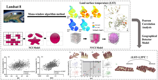
The Challenge of the Urban Compact Form: Three-Dimensional Index Construction and Urban Land Surface Temperature Impacts

Abstract

Cities are growing higher and denser, and understanding and constructing the compact city form is of great importance to optimize sustainable urbanization. The two-dimensional (2D) urban compact form has been widely studied by previous researchers, while the driving mechanism of three-dimensional (3D) compact morphology, which reflects the reality of the urban environment has seldom been developed. In this study, land surface temperature (LST) was retrieved by using the mono-window algorithm method based on Landsat 8 images of **amen in South China, which were acquired respectively on 14 April, 15 August, 2 October, and 21 December in 2017, and 11 March in 2018. We then aimed to explore the driving mechanism of the 3D compact form on the urban heat environment (UHE) based on our developed 3D Compactness Index (VCI) and remote sensing, as well as Geo-Detector techniques. The results show that the 3D compact form can positively effect UHE better than individual urban form construction elements, as can the combination of the 2D compact form with building height. Individually, building density had a greater effect on UHE than that of building height. At the same time, an integration of building density and height showed an enhanced inter-effect on UHE. Moreover, we explore the temporal and spatial UHE heterogeneity with regards to 3D compact form across different seasons. We also investigate the UHE impacts discrepancy caused by different 3D compactness categories. This shows that increasing the 3D compactness of an urban community from 0.016 to 0.323 would increase the heat accumulation, which was, in terms of satellite derived LST, by 1.35 °C, suggesting that higher compact forms strengthen UHE. This study highlights the challenge of the urban 3D compact form in respect of its UHE impact. The related evaluation in this study would help shed light on urban form optimization.

1. Introduction

The urban form plays an important role in the accommodation of human urban activities and has changed greatly during a period of rapid urbanization. One obvious change is the expansion of urban land to support rapidly growing urban populations. The urban population accounted for 55% of the world’s population in 2018 and is expected to grow to 68% in 2050 according to the 2018 revision of World Urbanization Prospects [1].

Unlimited land expansion is not possible owing to limited land resources. Urbanization is accelerating and the living standards of people are improving, while the current state of the urban environment should also meet the needs of sustainable development [2]. Intensive land use and a compact urban form have been suggested for the sustainable development of urban areas, which means high density and high diversity would be an effective urban frame [3].

There have been many studies on different compact urban forms since the 1960s. It has been concluded that the urban compact form has both benefits and challenges. Some scholars believe that urban morphology and its regulation are beneficial. The compact urban form contains a large population with short transportation and communication distances, which benefits infrastructure efficiency [4], environmental pollution reduction, and ecosystem maintenance [5]. For instance, a compact urban form centralizes public service facilities within walking distance, making public facilities more accessible [6]. The Barcelona Superblock model reconfiguration of the urban compact form and transport structures can help a city become greener and more resilient to climate change [7]. Therefore, some technologies and strategies have been provided to optimize urban form through compactness method [8,9]. However, the compact urban form also has challenges from the point of view of land use and land cover changes [10]. These are mainly reflected in the following aspects: The compact environment results in a street canyon effect and urban local climate change, which will strengthen the urban heat environment (UHE) and increase building energy consumption. For example, excessive building density deteriorates UHE, resulting in more energy consumption and carbon emissions [11,12]. Household building energy consumption grows with city compactness [13].

The urban heat island (UHI) is defined by a higher air and surface temperature in urban area relative to their rural surroundings. The land surface temperature (LST) is a strong indicator of the UHI that is known as surface UHI (SUHI): There are LST differences between urban suburban and nearby rural areas. Thermal infrared remote sensing represents the main technical approach for estimating LST [14]; the urban heat environment (UHE) is a physical environment system with urban surface temperature and urban air temperature as the core [15,16]. In the present study, the research scope of the urban heat environment includes surface urban heating (land surface temperature) and atmospheric urban heating (air temperature). The urban heat environment (UHE) is determined by the energy balance of the urban area. Thus, different land covers, which have different geometry and thermophysical properties, play an important role in the UHE. For surface urban heating, studies have shown that variations in the land surface temperature (LST) were highest for an urban morphology of low-density and mid-height buildings and lowest for arrays of high-rise and high-density buildings [17]. In most cities, increased impervious surfaces and low tree cover densities represent the main driving processes that increase summer daytime surface urban heating intensity [14]. There has been a significant negative relationship between LST and the mean patch size and shape index of the patches of green space in Bei**g, China [18]. Similarly, there were also significant relationships between mean LST and the mean patch size and mean shape index of the patches of impervious surface (positive) and green space (negative) in the Gwynns Falls watershed, Maryland, USA [19]. Future populations in compact cities will be at greater risk of UHE under ongoing fast rapid urbanization processing [20,21]. Dramatic urbanization has led to obvious urban heat phenomenon worldwide. The urban heat phenomenon has become an important issue of the urban natural and built environment that largely impacts on the urban ecology, building energy consumption, and human comfort and health [22]. With regards to the effect on energy consumption, the urban heat environment could play a different role during the heating and cooling seasons [23,24]. For example, on average, street canyons could experience a temperature rise of 2 °C in summer; the maximum warming effect is 4 °C in compact high-rise areas of Hong Kong. The high temperature in summer would directly affect thermal comfort and overall quality of urban life, and it especially has a negative effect on summer habitat comfort because air conditioning systems increase cooling energy consumption and release a higher heat flux from the building to the outdoor air [25]. However, cities embrace their UHE as shields from extreme cold, and they provide considerable benefits in wintertime. The effect could be considered positive from the point of view of reducing heating energy consumption in winter [26]. Would compactness interventions have an impact on UHE? To answer this question, it is important to investigate the driving mechanism between UHE and the urban compact form [27].

Previous studies found that there were two ways of measuring the urban compact form, one based on comprehensive statistics of multi-index and the other based on urban space’s morphological characteristics. The former is similar to the indicator system for measuring urban sprawl proposed by Galster [28], or the four indicators proposed by Yu-Hsin Tsai that characterized urban compactness [29]. The ratio between the number of Point of Interests (POIs) within the study area and the patch size of the study area cloud can also be used to measure the compactness of urban spatial structures [30]. The latter can also be indicated by the sky view factor (SVF), building density, and floor area ratio (FAR) [31]. SVF has been widely used to measure the visible sky of streets and urban geometry, which is a micro-scale parameter that is computed as the ratio of the vertical visible sky within a given reference circle [32]. Thinh et al. used Newton’s law of universal gravitation to construct a two-dimensional (2D) compactness index [33]. They applied geographic information technology to urban land gridding and calculated the average gravitation between each pair of urban land grids. As the spatial gravity strengthens, the urban spatial compactness increases and the urban spatial structure becomes more compact. In order to eliminate the scale discrepancies among cities, Zhao et al. constructed a Normalized 2D Compactness Index (NCI) of the urban compact form by using a contrasted circle that had the same urban construction area [34]. An NCI is thus more scientific for comparing the degrees of compactness of different cities [35]. There are also a variety of landscape metrics that were used to quantify the compactness of cities, such as the mean patch fractal dimension and the mean shape index [36]. The fractal dimension of urban agglomerations is also a measure of their compactness, i.e., compact cities usually have large values of fractal dimension [37]. Similarly, the landscape shape index has been used as a potential indicator of urban form development in landscape ecology worldwide and was introduced to indicate the divergence of the shape of a landscape patch from a circle that is considered ideal [38]. The shape index as an urban morphology element was also applied to each individual cool- and hot-spot feature, with the aim of providing a measurement of geometrical complexity of the hot-spot pattern. A recent study found that the shape index value of the extreme level was closely related to square or circular geometries, revealing that the highest average LST value of the study area was associated with a more regular shape than the corresponding cool-spot level [39].

However, the above methods included sky view factor (SVF), building density, landscape metrics, and Normalized 2D Compactness Index, which mostly analyzed the compactness of the 2D urban form. In reality, urban form is shown as three-dimensional; the vertical dimension could not be ignored for urban compact form construction. As urbanization continues, urban areas are not only growing denser, but are also growing higher. Thus, 2D urban form is not enough to capture the real urban compactness, while three-dimensional (3D) compactness is needed to accurately measure the form of the real city [40]. At the same time, UHE changes along with the development of urbanization. It is of great importance to precisely construct a compactness form in 3D and explore how the 3D compact morphology effects UHE. Therefore, we developed the Normalized 3D Compactness Index (NVCI) based on previous breakthroughs of the Normalized 2D Compactness Index (NCI), as well as the Law of Gravitation [41]. Then, based on the 3D compactness form and the NVCI model, the driving mechanism between urban 3D compactness and UHE would be improved.

Previous studies have highlighted the importance of factors related to the urban compact form and, in general, of geographical characteristics of cities (such as distance from the sea or from large water bodies) in the study of the UHE. Because the mitigation effect of the sea, i.e., sea breeze, the surface urban heating was always less intense and less evident in coastal metropolitan cities than in inland ones, though little attention has been paid to coastal cities [14]. However, the surface urban heat in coastal cities could not be ignored due to their unique geographical location and climatic conditions. The sea is likely to play a role in mitigating surface urban heating, as the temperature variations in water are relatively small compared to built-up areas [42]. In this study, using the Thermal Infrared Sensor (TIRS) on-board Landsat 8, we derived the LST from the five Landsat 8 images of the coastal city of **amen’s central urban area, acquired respectively on 14 April, 15 August, 2 October, and 21 December in 2017, and 11 March in 2018. The objectives of the present study are: (1) To evaluate the driving mechanism of urban 3D compact form on the UHE in example central urban areas of the coastal city of **amen, P.R. China, by using our developed 3D compact model based on Newton’s law of universal gravitation, geographical information system (GIS), remote sensing, and geo-detector and statistical analysis methods. (2) To demonstrate the advantage of 3D compact form by comparing it with 2D compact form. An understanding about how the urban 3D compact form effects UHE will contribute to improving the UHE and help to build a sustainable urban form.

2. Study Area

The research area, **amen, is a coastal island city on the southeastern coast of China, which is known for good habitat and rapid urbanization (Figure 1) [43]. The urbanization rate in this city was only 64% in 1980 but quickly grew to 86% in 2007. In 2019, the urbanization rate reached 89.2%, which was much higher than the national average of 46.4% across China [44]. Simultaneously, **amen is a hot summer and warm winter zone of coastal location that has a monsoonal humid subtropical climate, with mild winters and hot, rainy, and muggy summers. Rainfall is around 1200 millimeters per year, which is a little less rainy than the neighboring provinces (Zhejiang and Guangdong). The spring is from March to May and the hot season is in June, July, August, and September. The winter is from December to February. On average, the warmest month is July and the coolest months are December and January. The average annual maximum and minimum temperature are 25.0 °C and 18.0 °C, respectively [45,46]. We found that UHE intensity increased with the increments of built-up areas in our previous study on **amen city. Meanwhile, built-up area had positively correlated with urban warming [44]. Because of the rapid urbanization and typical coastal city climate, **amen is ideal for the study of the relationship between urban 3D compact form and UHE. The results can provide sustainable urban construction recommendations for similar coastal cities, which accommodate more than 50% of the world population [47]. In the present work, we expand upon our previous study area of **amen Island and cover a large part of the mainland. The four districts of Huli, Siming, Jimei, and Haicang, which are economic and political centers, and account for 74.89% of the total population of **amen, were chosen as the case study area.

3. Research Design and Data Collection

3.1. Indicator of Urban Compactness

Over the past five decade, measurements for a compact city have been mainly based on the 2D form. To fill in the gap and develop measurement of urban compactness, the 3D Compactness Index (VCI) and Normalized 3D Compactness Index (NVCI) have been proposed. These data were extracted by Remote Sensing (RS) and Geographic Information System (GIS) techniques.

3.1.1. Normalized 2D Compactness Index (NCI)

Thinh et al. proposed a quantitative measurement model (T model) to calculate urban compactness [33]. On the basis of GIS and urban land-use data, the T model overlays the grid cell of a certain size of urban land-use data to generate the basic data layer for model operation. As an example, Figure 2 shows the urban land-use data obtained from Landsat remote-sensing images, and the pixel size of the image is 30 m × 30 m. The grid cell size is 60 m × 60 m, which depends on the scale of the study region area of the urban construction land [34]. The T model can measure the 2D spatial gravity between different parts of urban construction land. The T model is expressed as follows:

$$\mathrm{CI}=\frac{{{\displaystyle \sum }}_{\mathrm{i}=1}^{\mathrm{n}}{{\displaystyle \sum }}_{\mathrm{j}=1, \mathrm{j}\ne \mathrm{i}}^{\mathrm{n}}\frac{1}{\mathrm{c}}\frac{{\mathrm{Z}}_{\mathrm{i}}{\mathrm{Z}}_{\mathrm{j}}}{{\mathrm{d}}^2\left(\mathrm{i},\mathrm{j}\right)}}{\mathrm{N}\left(\mathrm{N}-1\right)/2}$$

(1)

where CI is the 2D Compactness Index; the stronger the spatial gravitation, the more compact the urban form will be and the greater the CI is; hence, there is no range value of CI; i and j are two arbitrary grid cells in the study area; Z_i and Z_j are, respectively, areas of urban construction land (grey part in Figure 2) in urban grid cell i and j (i ≠ j); d (i, j) is the geometrical distance between the grid cell i and j (i ≠ j); and c is a constant (m², to make the calculation result of CI non-dimensional). The value of c depends on the size of the region in which we calculate the 2D Compactness Index; for example, the c value is usually small when we calculate the CI of communities (c = 100 m² in this study), while the c value will be large when we calculate the CI of the entire city or even a larger area. N is the total number of the urban construction land grid cells.

To offset the influence of the study area factor on the T model, the Normalized 2D Compactness Index (NCI) is presented as an improvement [34]. The Normalized 2D Compactness Index is defined as the ratio of the actual urban construction land to the equivalent circular land (Figure 3) [48]. It not only integrates various features of irregular urban form but also standardizes the calculation results, to compare compactness of different cities. Song et al. used NCI to research the relationships between urban commuting and urban form. The NCI model is expressed as follows [35]:

$$\mathrm{NCI}=\frac{ \mathrm{CI}}{{\mathrm{CI}}_{\max }}$$

(2)

where NCI is the Normalized 2D Compactness Index of which the value is between 0 and 1, CI is the 2D Compactness Index, and CI_max is the 2D Compactness Index of the equivalent circularity, i.e., the 2D urban form is more compact as NCI will approach 1.

3.1.2. Normalized 3D Compactness Index (NVCI)

The T model and NCI model are advanced measurements used to calculate 2D urban compactness. However, the realistic urban spatial form has a vertical dimension. To remedy the shortcoming that 2D compactness does not express the actual spatial form of cities, we proposed the 3D Compactness Index (VCI), which improved the 2D compactness model and is also based on Newton’s law of universal gravitation [41]. The VCI model can explain the total 3D spatial attractions of a city. A large VCI result indicates strong urban spatial attraction. The VCI model is expressed by Equation (3):

$$\mathrm{VCI}=\frac{{{\displaystyle \sum }}_{\mathrm{i}=1}^{\mathrm{n}}{{\displaystyle \sum }}_{\mathrm{j}=1, \mathrm{j}\ne \mathrm{i}}^{\mathrm{n}}\frac{1}{\mathrm{c}}\frac{{\mathrm{V}}_{\mathrm{i}}{\mathrm{V}}_{\mathrm{j}}}{{\mathrm{d}}^2\left(\mathrm{i},\mathrm{j}\right)}}{\mathrm{N}\left(\mathrm{N}-1\right)/2}$$

(3)

where VCI is the 3D Compactness Index of a specific urban space; a larger VCI indicates a more compact urban 3D form, hence there is no range value of VCI. V_i and V_j are, respectively, volumes of urban buildings in urban cube I and cube j (i ≠ j), (i, j) is the geometric distance between the centroids of urban cube i and cube j; the unit cube also depends on the scale of the study region and the volume of the urban buildings (Figure 4); c is constant (m⁴, to make the calculation result of VCI non-dimensional). The value of c depends on the size of the region in which we calculate the 3D Compactness Index; for example, the c value is usually small when we calculate the VCI of communities (c = 100 m⁴ in this study) while the c value will be large when we calculate the VCI of the entire city or even a larger area. N is the total number of cubes [41].

As shown in Formula (3), the VCI model is closely related to city scale. In order to eliminate errors caused by city scale differences, the Normalized 3D Compactness Index (NVCI) was proposed. We used a sphere as the maximum compactness form of 3D urban space and proposed the NVCI model. The Normalized 3D Compactness Index (NVCI) is calculated by the ratio of actual 3D urban spatial form to its equivalent sphere. The actual urban spatial form shares the same volume with its equivalent sphere (Figure 5). The compactness of various cities or different scales of urban area can be compared using the Normalized 3D Compactness Index (NVCI). The NVCI is given by:

$$\mathrm{NVCI}=\frac{ \mathrm{VCI}}{{\mathrm{VCI}}_{\max }}$$

(4)

where NVCI is the Normalized 3D Compactness Index and ranges between 0 and 1, while VCI is the 3D Compactness Index, and VCI_max is the 3D Compactness Index of the equivalent sphere; the closer the value of NVCI is to 1, the more compact the urban spatial form is [41].

3.2. Calculation of NCI and NVCI

We selected a typical coastal city, **amen, which is a subtropical city located in southeastern China, as the experimental area. The volumes of urban buildings that were used as factors of the VCI and NVCI models were combined with urban construction areas as well as building heights. We obtained the boundary of communities in **amen by vectorization method (i.e., using the polygon feature template in the Create Features window of Arc GIS to create polygons) based on GF-1 satellite remote-sensing images of **amen in 2017. We then used the 2017 Pléiades 50 cm global high-resolution satellite imagery as a reference to proofread and adjust the boundaries of communities in order to obtain more accurate boundary data. Based on 2017 aerial imagery of the **amen land survey, we used the object-based image analysis techniques to delineate building footprints, while zonal statistics was used to extract building height information. Then, we also proofread the buildings’ heights data through field surveys [49,50]. According to Formulas (3) and (4), we built an urban unit cube of 5 m × 5 m × 5 m and calculated the VCI and NVCI of each community by Python 2.7. Then, we also measured the average building height, building density, CI and NCI of all communities. Based on the above method and calculation results, we deleted the very small communities with only one building in order to ensure the accuracy of communities’ NVCI value. The experimental files comprised 841 communities (valid data) with different urban morphologies in **amen, southeastern China and were included in the final analysis (Figure 6). These communities are consistent with the boundary red line of residential communities, which is approved by the urban construction system.

3.3. Retrieval of Land Surface Temperature

The Landsat images we used were provided by the United States Geological Survey (https://www.usgs.gov/ accessed on 1 January 2021) for free. Although there are two thermal infrared bands in the Landsat 8 Operational Land Imager-Thermal Infrared Sensor (OLI-TIRS) data, the land surface temperature (LST) can be accurately inversed only by band 10. As we know, the thermal imagery from Landsat sensors, provided with relatively high spatial resolution, is suitable for monitoring the urban thermal environment. The TIRS thermal bands of Landsat 8 were acquired at 100 m resolution, but were resampled to 30 m in the delivered data product, and could then meet the urban communities’ research requirement [51].

The mono-window algorithm, an accurate method, was processed to retrieve the LST of **amen in the years 2017–2018. Five cloud-free Landsat 8 images were obtained for this study. They were acquired at approximately 10:43 a.m. (Bei**g time) on 14 Apr, 15 Aug, 2 Oct, and 21 Dec in 2017, and 11 Mar in 2018. Two steps were taken to retrieval LST: (1) converting the pixel values to at-sensor brightness temperatures; and (2) correcting for the spectral emissivity. Four parameters are critical for calculating LST: brightness temperature, ground emissivity, effective mean atmospheric temperature, and atmospheric transmittance, which could be acquired by Radiometric Calibration, normalized difference vegetation index (NDVI) (http://atmcorr.gsfc.nasa.gov/ accessed on 25 May 2020) (Formulas (5)–(11)),

$$C=\epsilon \tau$$

(5)

$$D=\left(1-\epsilon \right)\left[1+\left(1-\epsilon \right)\tau \right]$$

(6)

$$\tau =1.031412-0.115367w$$

(7)

$$\epsilon =0.02644F_v+0.96356$$

(8)

where $C$ and $D$ are empirical equations, which are related to the land surface emissivity and atmospheric transmittance, $\mathsf{\epsilon }$ is the land surface emissivity, $\tau$ is the total atmospheric transmittance, and $w$ is the total atmospheric water vapor content, which ranges from 1.6 to 3.0 [52].

$$F_v=\frac{NDVI-NDV{I}_{min}}{NDV{I}_{max}-NDV{I}_{min}}$$

(9)

$$NDVI=\left({\rho }_{nin}-{\rho }_{red}\right)/\left({\rho }_{nin}+{\rho }_{red}\right)$$

(10)

where $F_v$ is the vegetation proportion [53]; $NDV{I}_{max}$ and $NDV{I}_{min}$ are the maximum and minimum $NDVI$ values in the region, respectively; and ${\rho }_{nin}$ and ${\rho }_{red}$ are the reflectance values of the NIR and red channels (band 5, band 4, and for Landsat 8), respectively.

$$LST=\frac{a\left(1-C-D\right)+\left[b\left(1-C-D\right)+C+D\right]\times T_b-D\times T_a}{C}-237.15$$

(11)

$$T_b=\frac{K_2}{ln\left(K_1/L_b+1\right)}$$

(12)

$$L_b=L_{min}+\frac{L_{max}-L_{min}}{255}DN$$

(13)

where $LST$ is the land surface temperature; $T_a$ is the effective mean atmospheric temperature, which can be calculated from the near surface temperature during acquisition time of Landsat 8; and a and b are constant as −67.3554 and 0.4586, respectively, when the LST is between 0 °C to 70 °C [54]. $T_b$ is the effective brightness temperature at the sensor on remote-sensing satellite in Kelvin; $K_1$ and $K_2$ are empirical constants values. $K_1$ is $774.89 {\mathrm{mWcm}}^{-2}{\mathrm{sr}}^{-1}{\mathsf{\mu }\mathrm{m}}^{-1}$; $K_2$ is $1321.08 \mathrm{K}$; $L_b$ is the spectral radiance at the sensor’s aperture in ${\mathrm{Wm}}^{-2}{\mathrm{sr}}^{-1}{\mathsf{\mu }\mathrm{m}}^{-1}$; and $L_{min}$ and $L_{max}$ are the minimum and maximum radiances that can be detected by the sensor, respectively. $L_{min}$ and $L_{max}$ can be found in the header text file of the Landsat 8 raw data. LST maps for five dates are shown in Figure 7.

3.4. Geographical Detector Models Methods

The geographical detector model (GeoD) is composed of interactive, factor, ecological, and risk detectors, and is a spatial analysis model based on the theory of spatial heterogeneity and has been applied in many geographical and ecological studies [55]. It is freely available from http://www.geodetector.org/ (accessed on 1 January 2021). In this study, the interactive detector was used to explore the interaction of influencing factors (X) on the heat accumulation (Y), which includes 2D architectural factors such as Building Density (BD); Normalized 2D Compactness Index (NCI); and 3D architectural factors such as Building Height (BH) and Normalized 3D Compactness Index (NVCI). The factor detector was used to explore the impact of different explanatory variables X1, X2… on the research target, while the ecological detector was used to explore whether any two factors, X1 and X2, had different significant impacts on Y. Additionally, the risk detector was used to search for the range in which factors significantly affect LST variation, and q is the association between Y and X, which is measured by [56]:

$$q=1-\frac{1}{N{\sigma }^2}{\displaystyle \sum }_{h=1}^L{N}_h{\sigma }_h^2=1-\frac{SSW}{SST}$$

(14)

where ${\sigma }^2$ is the variance of Y; the study population of Y is composed of $L$ strata ($h=1, 2, 3 \dots L$); $N$ stands for the number of units in the study population of Y. The strata of Y may exist already, or are constructed by classification or formed by laying Y over X, which consists of strata. Here, we used the K-means method to convert explanatory factors from actual values into category variables [57]. $SSW$ and $SST$ is the within sum of squares and the total sum of squares, respectively. q∈[0,1]; the value of the q-statistic indicates how much Y is interpreted by X. In detail, $q$= 0 indicates there is no association between Y and X, while $q$= 1 means that Y is completely determined by X. The higher the q value, the stronger is the spatially stratified heterogeneity of Y [58].

The q value of the interaction between the factors (X1, X2…) will be calculated by the interaction detector, namely q (X1 ∩ X2). According to the relationship between q (X1), q (X2), and q (X1 ∩ X2), the interaction can be divided into nonlinear weaken, single-factor nonlinear weaken, independent, double-factor enhancement, and nonlinear enhancement (

Table 1. Types of interaction between two variables.

Relationship	Interaction
q (X1 ∩ X2) < Min [q (X1), q (X2)]	nonlinear weaken (NW)
Min[q(X1), q(X2)] < q (X1 ∩ X2) < Max [q (X1), q (X2)]	single-factor nonlinear weaken (SNW)
q (X1 ∩ X2) > Max [q (X1), q (X2)]	double-factor enhancement (DE)
q (X1 ∩ X2) = q (X1) + q (X2)	independent (I)
q (X1 ∩ X2) > q (X1) + q (X2)	nonlinear enhancement (NE)

) [57,59].

4. Results

4.1. Urban Building Characteristics

Table 2. Statistics of urban building characteristics.

	Building Area (hm2)	Building Height (Floor)	Building Density (%)	2D Compact Indexes			3D Compact Indexes
				CI	CImax	NCI	VCI	VCImax	NVCI
Mean	4.856	9	35.781	1.82 × 10−3	2.61 × 10−3	0.622	0.016	0.334	0.044
Maximum	44.764	38	85.257	0.018	0.019	0.979	0.190	1.691	0.323
Minimum	0.044	1	10.198	4.14 × 10−5	9.14 × 10−5	0.370	2.42 × 10−4	0.063	1.45 × 10−3

shows the statistical results for the different buildings in **, and shadowing effects, a 3D compact form changes urban heating exchange and stocks, which are different from those only from land surface. Buildings act as blocks to reduce wind speed and alter wind profile in the canopy [64,65]. Moreover, high building envelopes affect the flow of sensible-heat flux, and the solar radiation processing varies accordingly [66,67]. The trap** of solar radiation causes energy to be stored in the urban building canyon as buildings become higher and streets narrower [68]. These have been confirmed to be the controlling factors in the relationship between the urban 3D compact form and UHE. Hence, a 3D compact form leads to prominent UHE stress due to its nature, more so than 2D compactness.

The impact of urban morphology on canopy temperature variations, mostly through radiation shadowing and trap**, has been well described [69,70], as has the heat storage [71,72]. In this study, because large spatial coverage air temperature measurements are not available, we used the land surface temperature (LST) from satellite images to discuss the impact of urban 3D compactness on the temperature variation.

Here we use a simple conceptual energy balance model to explain the observed correlations between LST and morphology. The surface temperatures, T, is determined by the surface energy balance [73,74]:

$$C\frac{dT}{dt}=Q_{SW}-Q_{LW}+Q_F-Q_H-Q_E$$

(15)

On the left hand, C is the effective thermal mass that is calculated as the production of density, ${\rho }_s$, specific heart, $c_s$, effective depth, $d_s$, and the total surface area$, A$.

$$C={\rho }_s{c}_s{d}_{s}A$$

(16)

On the right hand, $Q_{SW}$ is the solar short-wave radiation at the surface, $Q_{LW}$ is the outgoing long-wave radiation, $Q_F$ is the anthropogenic heat, and $Q_H$ and $Q_E$ are sensible heat flux and latent heat flux, respectively.

In this study, the LST mainly consists of the temperature from the horizontal surfaces, i.e., the ground and roof, while the vertical surfaces are usually excluded (Figure 13).

$$LST=BD\ast T_{s_{roof}}+\left(1-BD\right)\ast T_{s\_ground}$$

(17)

As the surface area for the total urban canopy (ground and wall) are larger than the roof area, this will result in a much larger thermal mass. Together with the shading effect, the surface temperature in the roof, $T_{s\_roof}$, is usually higher than at the ground, $T_{s\_ground}$ in the daytime. At night, however, due to its large sky view factor and stronger wind in the roof, which result in stronger nocturnal cooling through long wave radiation and convection, $T_{s\_roof}$ is usually lower than the ground $, T_{s\_ground}$. Thus, when increasing the building density (BD), daytime LST would be higher, which is resulted from an overall effect of canyon geometry on solar radiation. Our results were consistent with the findings of Guo et al., who found that building density had a stronger effect than building height on the LST [17]. The difference was that they believed that an urban morphology of a medium building height and lower density yielded a higher heat accumulation. Moreover, the land cover of the ground surface also plays a role. For instance, compared with impervious surfaces, the green areas would absorb less solar radiation due to relatively higher albedo and stronger cooling latent heat cooling, and $T_{s\_ground}$ would be less. Besides, there are other meteorological and geographical factors, such as cloud, rainfall, anthropogenic heat, etc., that have an impact on the surface energy balance as well as the LST. However, any radiometer at a fixed position has a biased view when observing a convoluted, three-dimensional surface such as an urban canopy. A methodology based on a panoramic time sequential thermography data set is important for the calculation of the complete surface temperature [75]. Surface emissivity over urban areas is also critical in surface temperature estimation and is related to energy budget. In order to match urban studies, improving the estimation of urban surface emissivity is essential [76]. Hence, the exact mechanism between urban 3D compact form and LST and the contributions of these factors may need further study.

These could also explain the seasonal variations between NVCI and UHE in Section 4.4. The seasonal discrepancies in the impact of urban 3D compactness on LST is largely subject to the interactions between canyon geometry and incoming solar radiation, i.e., radiation trap** and shadowing effects that are related to the geographic location and solar angle. In general, increasing the compactness can enhance both the shadowing and the trap** effects. The trap** effect supports the UHE, whereas shadowing effects reduce the UHE, resulting in a nonlinear impact of canyon geometry and solar angle on UHE [69,70].

This study was conducted in **, and shadowing effects. The driving process of the urban 3D form on UHE was further proved by different urban morphology types. Individually, building density had a greater effect on UHE than building height. Despite this, the vertical scale should not be ignored due to the enhanced UHE when including the two factors of ‘height’ and ‘density’.

(3)

Temporal and spatial UHE heterogeneity is driven by a 3D compact form. In areas with warm winters and hot summers, a positive correlation between urban 3D compactness and LST was observed in the warm season, while a negative correlation was observed in the cold season. The 3D compact form has more prominent UHE stress in autumn than other seasons due to its horizontal and vertical element integration, as well as radiation trap** effects.

(4)

The Normalized 3D Compactness Index (NVCI) levels were accessed with high confidence to reveal that dominant factors in special categories had a high ability to increase heat accumulation. Increasing the 3D compactness of an urban community from level 3 to level 1 (0.016–0.323) would increase the heat accumulation by 1.35 °C, which is also equivalent to increasing the average building density from 31.84% to 51.74%, or increasing average building height from 8 floors to 11 floors. This means that the compact urban 3D form is not always better. A too compact form will strengthen UHE.

Although our research confirmed that the urban 3D compact form has a significant effect on the UHE, some limitation still exits: (1) For the retrieval of LST, the satellite sensors do not measure the complete surface temperature. It would be more accurate to use a methodology that could be applied to simulate the measurement bias of different remote sensors when inferring longwave emittance and surface temperature of a convoluted, three-dimensional urban surface [75]. Because NDVI emissivity corrections for LST are not suitable for urban studies, how the urban 3D form affects the land surface emissivity is worth discussing, particularly topics such as improving the estimation of urban surface emissivity based on spectral mixture analysis [76]. Moreover, the dense time series of LST is also useful for obtaining convincible conclusions on LST characteristics. (2) The LST is different from the air temperature, which has a great influence on determining human thermal comfort in urban areas [17]. Thus, high resolution on-site air temperature observation and numerical modelling data would be helpful to further verify the obtained results from remote-sensing images. (3) Apart from the buildings and their geometry, other urban landscape elements such as vegetated areas (starting from grass to trees) also play a potential role in the urban heat environment (UHE). Urban tree and green infrastructures are now widely considered as an effective way to mitigate urban heating. An integration of 3D building geometry and green areas and infrastructures would be essential to the holistic approach for improving the urban heat environment. (4) The proposed NVCI is applicable at both community and urban scales. The scale of this study was limited to the urban community level. In future, a comparative study of different urban form indictors (e.g., NVCI, SVF) in China’s larger cities and even mega-cities throughout the world under different climatic conditions, together with different variables (tree cover, water body…), would be of great interest in order to explore their impact on urban heat environment. In addition, we believe the urban 3D compact model could be considered in many other areas of research, such as the urban 3D compact form influencing urban atmospheric pollution transfer [77]. It is also important to provide scientific guidance for climate response urban planning in cities in terms of different latitudes and climatic backgrounds, promoting a healthier and more sustainable urban habitat.

References

1. United Nations. World Urbanization Prospects: The Revision; United Nations: New York, NY, USA, 2018. [Google Scholar]
2. Ye, H.; Wang, K.; Huang, S.; Chen, F.; ** with aerial imagery and GIS data. Int. J. Appl. Earth Obs. 2011, 13, 841–852. [Google Scholar] [CrossRef]
3. Chen, F.; Yang, S.; Yin, K.; Chan, P. Challenges to quantitative applications of Landsat observations for the urban thermal environment. J. Environ. Sci. China 2017, 59, 80–88. [Google Scholar] [CrossRef] [PubMed]
4. Artis, D.A.; Carnahan, W.H. Survey of emissivity variability in thermography of urban areas. Remote Sens. Environ. 1982, 12, 313–329. [Google Scholar] [CrossRef]
5. Sobrino, J.A.; Jiménez-Muñoz, J.C.; Paolini, L. Land surface temperature retrieval from LANDSAT TM 5. Remote Sens. Environ. 2004, 90, 434–440. [Google Scholar] [CrossRef]
6. Qin, Z.; Karnieli, A.; Berliner, P. A mono-window algorithm for retrieving land surface temperature from Landsat TM data and its application to the Israel-Egypt border region. Int. J. Remote Sens. 2001, 22, 3719–3746. [Google Scholar] [CrossRef]
7. Wang, J.F.; Li, X.H.; Christakos, G.; Liao, Y.L.; Zhang, T.; Gu, X.; Zheng, X.Y. Geographical Detectors-Based Health Risk Assessment and its Application in the Neural Tube Defects Study of the Heshun Region, China. Int. J. Geogr. Inf. Sci. 2010, 24, 107–127. [Google Scholar] [CrossRef]
8. Ye, H.; Hu, X.; Ren, Q.; Lin, T.; Li, X.; Zhang, G.; Shi, L. Effect of urban micro-climatic regulation ability on public building energy usage carbon emission. Energy Build. 2017, 154, 553–559. [Google Scholar] [CrossRef]
9. Hu, Y.; Wang, J.; Li, X.; Ren, D.; Zhu, J. Geographical Detector-Based Risk Assessment of the Under-Five Mortality in the 2008 Wenchuan Earthquake, China. PLoS ONE 2011, 6, e21427. [Google Scholar] [CrossRef] [PubMed] [Green Version]
10. Zhang, J.; Yu, L.; Li, X.; Zhang, C.; Shi, T.; Wu, X.; Yang, C.; Gao, W.; Li, Q.; Wu, G. Exploring Annual Urban Expansions in the Guangdong-Hong Kong-Macau Greater Bay Area: Spatiotemporal Features and Driving Factors in 1986–2017. Remote Sens. 2020, 12, 2615. [Google Scholar] [CrossRef]
11. Wang, J.; Xu, C. Geodetector: Principle and prospective. Acta Ecol. Sin. 2017, 72, 116–134. [Google Scholar]
12. **amen Municipal Bureau of Natural Resources and Planning. **amen City Planning Management Technical Regulations; **amen Municipal Bureau of Natural Resources and Planning: **amen, China, 2010.
13. Alavipanah, S.; Schreyer, J.; Haase, D.; Lakes, T.; Qureshi, S. The effect of multi-dimensional indicators on urban thermal conditions. J. Clean. Prod. 2018, 177, 115–123. [Google Scholar] [CrossRef]
14. Scarano, M.; Mancini, F. Assessing the relationship between sky view factor and land surface temperature to the spatial resolution. Int. J. Remote Sens. 2017, 38, 6910–6929. [Google Scholar] [CrossRef]
15. Ye, H.; Sun, C.; Wang, K.; Zhang, G.; Lin, T.; Yan, H. The role of urban function on road soil respiration responses. Ecol. Indic. 2018, 85, 271–275. [Google Scholar] [CrossRef]
16. Unger, J. Intra-urban relationship between surface geometry and urban heat island: Review and new approach. Clim. Res. 2004, 27, 253–264. [Google Scholar] [CrossRef] [Green Version]
17. Caton, F.; Britter, R.E.; Dalziel, S. Dispersion mechanisms in a street canyon. Atmos. Environ. 2003, 37, 693–702. [Google Scholar] [CrossRef]
18. Emmanuel, R.; Rosenlund, H.; Johansson, E. Urban shading—A design option for the tropics? A study in Colombo, Sri Lanka. Int. J. Climatol. 2007, 27, 1995–2004. [Google Scholar] [CrossRef] [Green Version]
19. Eliasson, I. Urban nocturnal temperatures, street geometry and land use. Atmos. Environ. 1996, 30, 379–392. [Google Scholar] [CrossRef]
20. Yang, X.; Li, Y. The impact of building density and building height heterogeneity on average urban albedo and street surface temperature. Build. Environ. 2015, 90, 146–156. [Google Scholar] [CrossRef]
21. Theeuwes, N.; Steeneveld, G.; Ronda, R.J.; Heusinkveld, B.; Hove, B.; Holtslag, B. Seasonal Dependence of the Urban Heat Island on the Street Canyon Aspect Ratio. Q. J. R. Meteor. Soc. 2014, 140, 2197–2210. [Google Scholar] [CrossRef]
22. Song, J.; Wang, Z. Interfacing the Urban Land-Atmosphere System Through Coupled Urban Canopy and Atmospheric Models. Bound. Layer Meteorol. 2015, 154, 427–448. [Google Scholar] [CrossRef]
23. Wang, K.; Li, Y.; Li, Y.; Lin, B. Stone forest as a small-scale field model for the study of urban climate. Int. J. Climatol. 2018, 38, 3723–3731. [Google Scholar] [CrossRef]
24. Chen, G.; Wang, D.; Wang, Q.; Li, Y.; Wang, X.; Hang, J.; Gao, P.; Ou, C.; Wang, K. Scaled outdoor experimental studies of urban thermal environment in street canyon models with various aspect ratios and thermal storage. Sci. Total Environ. 2020, 726, 138147. [Google Scholar] [CrossRef]
25. Oke, T.R.; Mills, G.; Christen, A.; Voogt, J.A. Urban Climates; Cambridge University Press: Cambridge, UK, 2017. [Google Scholar]
26. Wang, K.; Li, Y.; Wang, Y.; Yang, X. On the asymmetry of the urban daily air temperature cycle. J. Geophys. Res. Atmos. 2017, 122, 5625–5635. [Google Scholar] [CrossRef]
27. Adderley, C.; Christen, A.; Voogt, J.A. The effect of radiometer placement and view on inferred directional and hemispheric radiometric temperatures of an urban canopy. Atmos. Meas. Tech. 2015, 8, 2699–2714. [Google Scholar] [CrossRef] [Green Version]
28. Mitraka, Z.; Chrysoulakis, N.; Kamarianakis, Y.; Partsinevelos, P.; Tsouchlaraki, A. Improving the estimation of urban surface emissivity based on sub-pixel classification of high resolution satellite imagery. Remote Sens. Environ. 2012, 117, 125–134. [Google Scholar] [CrossRef]
29. Abbassi, Y.; Ahmadikia, H.; Baniasadi, E. Prediction of pollution dispersion under urban heat island circulation for different atmospheric stratification. Build. Environ. 2020, 168, 106374. [Google Scholar] [CrossRef]
Figure 1. Location of the study area.
Remotesensing 13 01067 g001
Figure 2. Grids in two-dimensional (2D) urban compactness model [34].
Remotesensing 13 01067 g002
Figure 3. Urban construction land and its equivalent circular land [34].
Remotesensing 13 01067 g003
Figure 4. Schematic diagram of the spatial cube division of three-dimensional (3D) urban space [41].
Remotesensing 13 01067 g004
Figure 5. Urban buildings and their equivalent volume sphere [41].
Remotesensing 13 01067 g005
Figure 6. Distribution of typical communities and urban buildings.
Remotesensing 13 01067 g006
Figure 7. Land surface temperature (LST) images in five different dates.
Remotesensing 13 01067 g007
Figure 8. (a) The building heights in communities with the maximum NVCI; (b) The building heights in communities with the minimum NVCI.
Remotesensing 13 01067 g008
Figure 9. Spatial distribution of the heat accumulation in each community of the study area, (a). Spatial distribution of the LST across four seasons in each community of the study area, (b).
Remotesensing 13 01067 g009aRemotesensing 13 01067 g009b
Figure 10. Relationship between heat accumulation and (a) NCI; (b) NVCI.
Remotesensing 13 01067 g010
Figure 11. The top panel shows the four typical urban morphology types of LL, HL, LH, and HH (ad); (e) Relationship between heat accumulation and average NVCI of four types.
Remotesensing 13 01067 g011
Figure 12. Relationships between NVCI and LST in (a) spring; (b) summer; (c) autumn; (d) winter.
Remotesensing 13 01067 g012
Figure 13. Simple schematic depiction of the main energy exchange fluxes comprising the surface energy balance of roof and urban canyon facets (a) by summer and (b) by winter. The structure of an urban canopy model, which simulates exchanges at street, wall, and roof surfaces representative of parts of a city.
Remotesensing 13 01067 g013