2.6. Estimation of the Crop Water Use
The green (CWU
G) and blue (CWU
B) portions of the crop water use (CWU) were calculated by accumulating the daily recorded evapotranspiration (ET, mm d
−1) for the entire growth period, following the procedure described by Allen et al. [
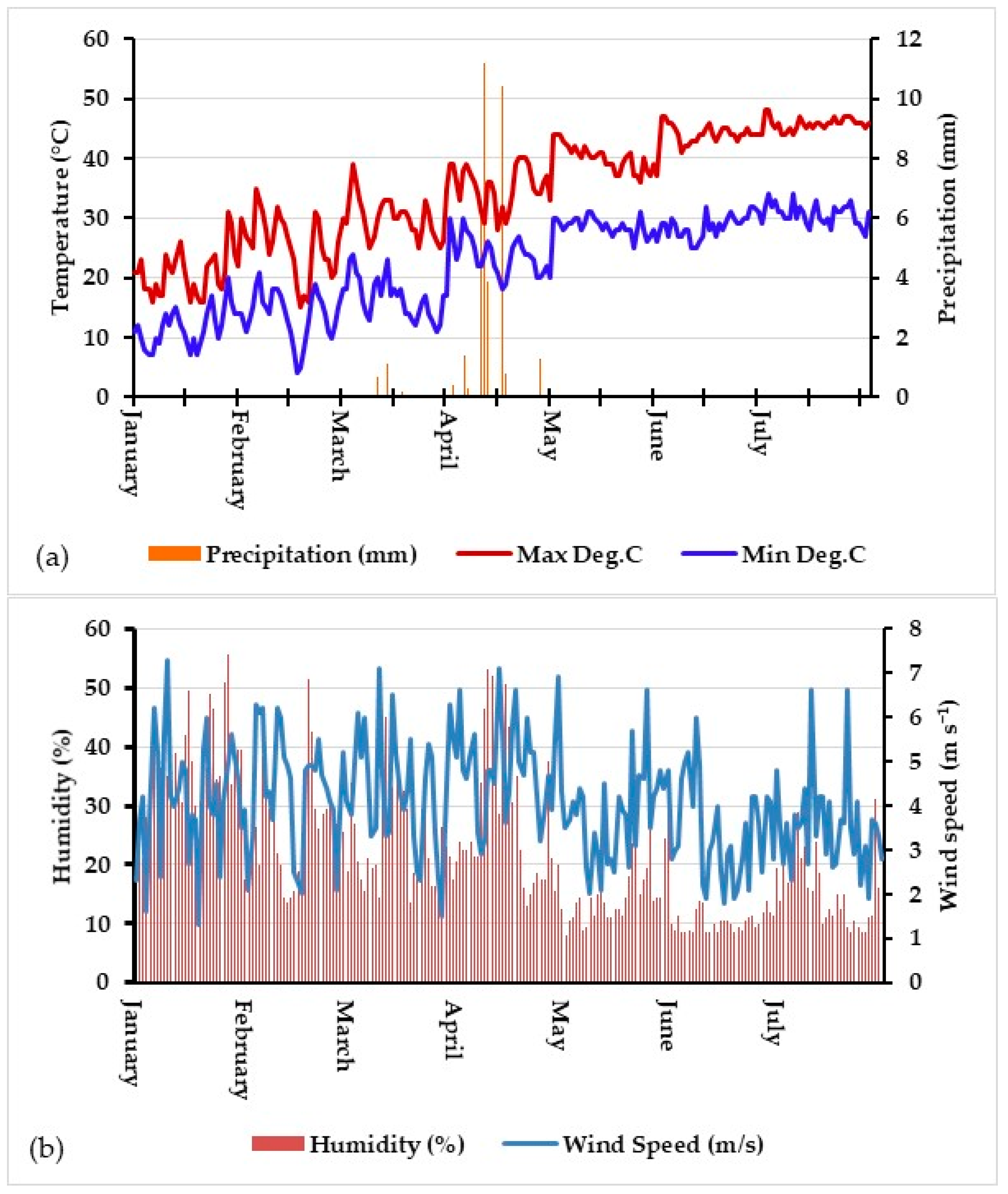
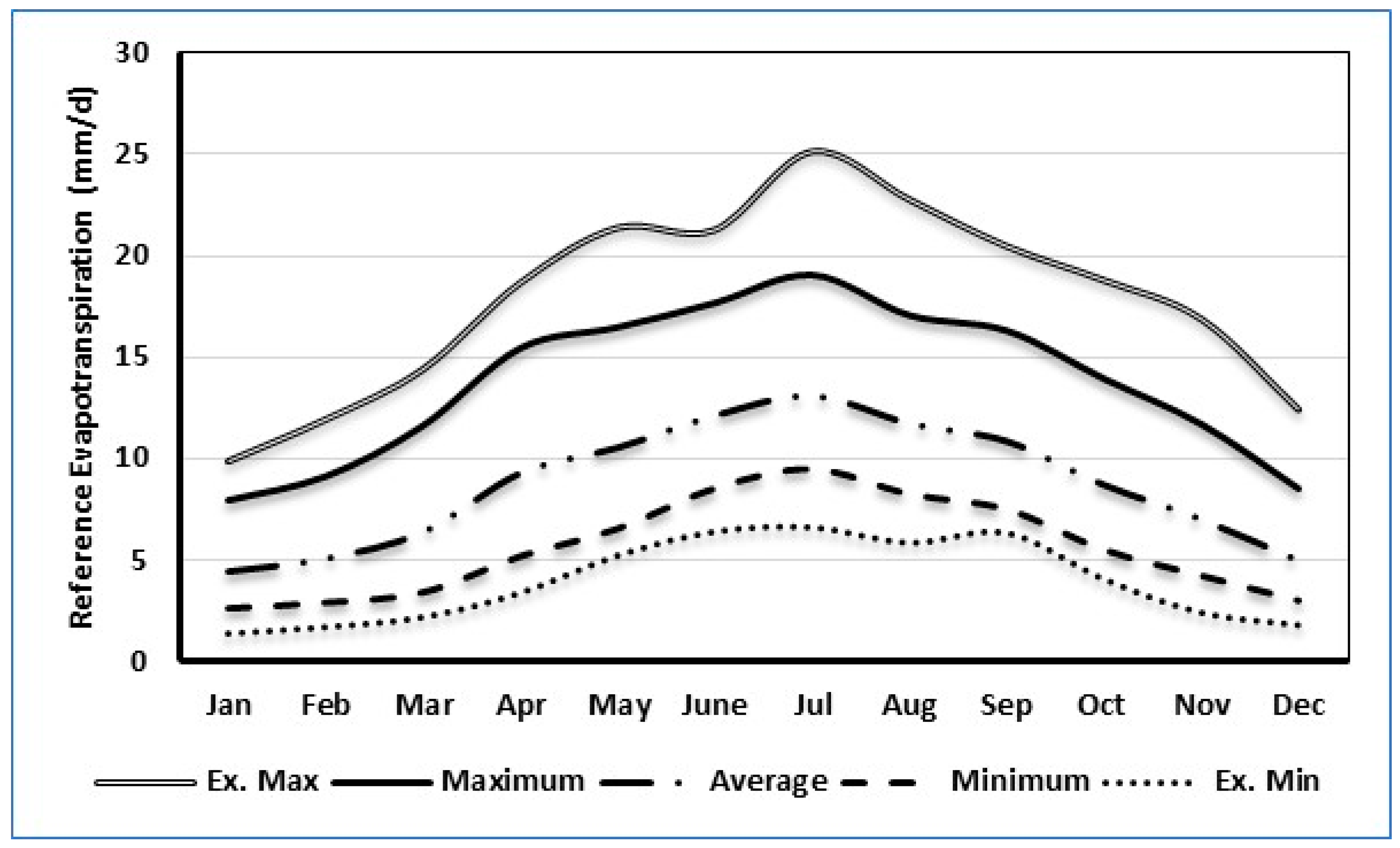
23]. The evaporative demand of the atmosphere (ET
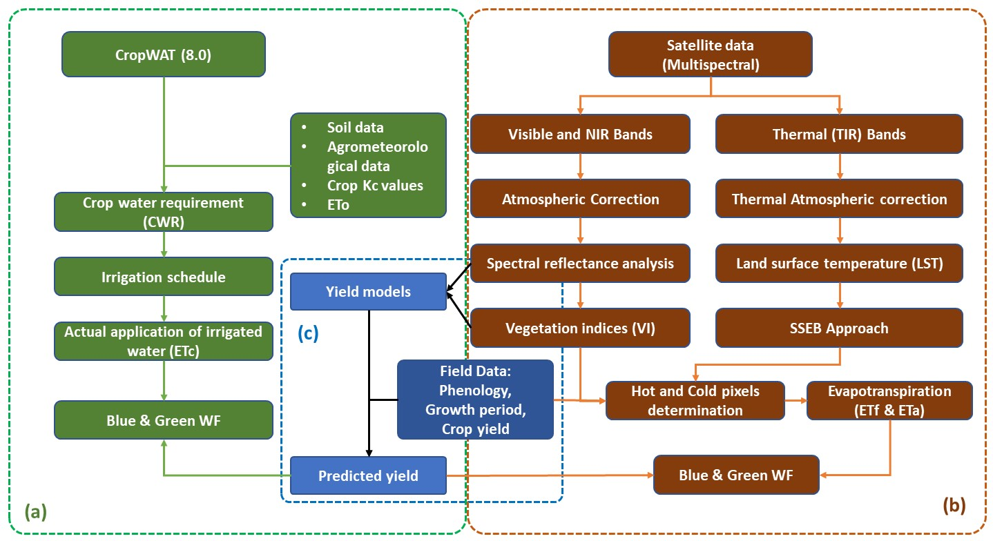
o) was determined using the standard Penman–Monteith method revised and recommended by the FAO. The CROPWAT model, which was used to calculate evapotranspiration, offers two different options for calculating evapotranspiration, i.e., the option of crop water requirements considering optimum constraints, and the option of irrigation practices, such as determining in real time the actual irrigation supply. For a remote sensing quantification of ET, the SSEB technique reported by Senay et al. [
14] was used to estimate the CWU as actual evapotranspiration (ET
a). The ET
a was obtained in two steps, namely, the estimation of reference ET fraction (ET
f) and the reference ET (ET
o) as shown in Equations (3)–(5).
where α is the scale element, usually 1.2. The reference evapotranspiration (ET
o) was determined after the FAO–Penman–Monteith method (Equation (5)), according to Allen et al. [
23]:
where:
ETo = reference evapotranspiration (mm day−1),
Rn = net radiation at the crop surface (MJ m−2 day−1),
G = soil heat flux density (MJ m−2 day−1),
T = air temperature at 2 m height (°C),
u2 = wind speed at 2 m height (m s−1),
es = saturation vapor pressure (kPa),
ea = actual vapor pressure (kPa),
es = ea saturation vapor pressure deficit (kPa),
Δ = slope vapor pressure curve (kPa °C−1),
γ = psychrometric constant (kPa °C−1)
ET
f is the key variable in the SSEB approach because it takes into account the effect of soil moisture on ET
a. ET
o determines a potential ET under unconstrained watering conditions. ET
f was computed using temperature datasets (LST and air), considering that hot pixels (T
h) experience little or no ET [
24,
25]. Cold pixels (Tc) represent the highest ET. Both S2 and L8 images were utilized to map the ET
f. In this study, however, vegetation coverage was calculated using the S2 data, and the LST was calculated using the TIRS bands of the L8 data.
Cloud-free Landsat-8 OLI/TIRS images were subjected to radiometric correction (linear contrast stretching) to reduce interference errors. The processed images were then used to calculate the crop evapotranspiration (ETc) through several computational stages including the brightness temperature (Tb), surface temperature (Ts), net radiation (Rn), geothermal flux (G), air heat flux (H), latent heat flux (LE), and finally the evapotranspiration using a digital image processing module (i.e., the SSEB).
The surface temperature (T
s) of each pixel was examined, and the determined hot and cold pixels were used for the calculation of the fraction of ET. Hot pixels were selected, using the NDVI map as a guide, by locating dry bare land (or sparse vegetation) with very low NDVI values. Similarly, cold pixels were selected from areas of high moisture, healthy, completely covered with vegetation, and with maximum values of NDVI. The ET fraction (ET
f,x) of an individual pixel (x) was also calculated using Equation (6):
where:
dTh = the temperature difference between the L8 estimated surface temperature (Ts) and the hot pixel air temperature (Ta).
dTc = the temperature difference between L8 estimated Ts and cold pixel Ta.
dTx = the temperature difference between Ts and Ta.
Ground temperatures of the six selected pixels (three hot and three cold) were estimated using the ArcGIS software, ver. 10.7.1 (ESRI, Redlands, CA, USA). The database file of the 9.0 software results was exported to an Excel (Microsoft, Redmond, WA, USA) spreadsheet, and then, the hot and cold pixels were averaged. Images containing the ETf of individual pixels were then utilized to calculate the ETa across the study period.
The green CWU (CWU
G) and blue CWU (CWU
B) for each crop were calculated following the method described by Hoekstra et al. [
3], as in Equations (7) and (8). ET
G and ET
B represent the green and blue water evapotranspiration, respectively, from the first day (d = 1) to the end of the growing season (lgp). The factor of 10 is to convert the water depth to millimeters, and then to water volume per land area (m
3 ha
−1).
ETG and ETB are the evapotranspiration (mm) by crops with respect to the green and blue components of the crop water footprint, respectively.
2.7. Assessment of Crop Water Footprint
The total water consumption (WF, m
3 t
−1) of a crop is the sum of the blue and green components of the WF, as shown in Equations (9)–(11) (Hoekstra et al., 2011). Both the blue and green WFs for a given crop was calculated by dividing the crop water consumption (CWU, m
3 ha
−1) by the crop productivity (CP, t ha
−1):
where WF
B and WF
G are the blue and green water footprint, CWU
G and CWU
B are the crop consumption of green (precipitation) and blue (surface and groundwater) water, and CP is the crop productivity (yield) based on the crop’s water demand and actual transpiration output from the CROPWAT/SSEB model.
WF
B is calculated based on field data as the amount of irrigation water applied is considered blue water, as given in Equation (12) [
26]:
where WF
MB (m
3 t
−1) is the WF
B calculated from the recorded irrigation data, Y
f is the crop yield (carrots and onions), I
r is the amount of water used throughout the irrigation season (mm), DP is the deep percolation of water out of the root zone (mm), and RO is the surface runoff. Since measuring losses in such large fields is challenging, an average irrigation efficiency of 70% was used for center pivot irrigation systems to account for total losses due to runoff, surface flow, and deep percolation [
27]. The total crop water requirement for the studied crops was estimated at 1940 mm and 824 mm for carrots and onions, respectively. However, the total volume of water used to irrigate the crops was 2658 mm and 1199 mm for carrots and onions, respectively.

 ,
, 


