DRL-Based Dynamic Destroy Approaches for Agile-Satellite Mission Planning

Abstract

Agile-satellite mission planning is a crucial issue in the construction of satellite constellations. The large scale of remote sensing missions and the high complexity of constraints in agile-satellite mission planning pose challenges in the search for an optimal solution. To tackle the issue, a dynamic destroy deep-reinforcement learning (D3RL) model is designed to facilitate subsequent optimization operations via adaptive destruction to the existing solutions. Specifically, we first perform a clustering and embedding operation to reconstruct tasks into a clustering graph, thereby improving data utilization. Secondly, the D3RL model is established based on graph attention networks (GATs) to enhance the search efficiency for optimal solutions. Moreover, we present two applications of the D3RL model for intensive scenes: the deep-reinforcement learning (DRL) method and the D3RL-based large-neighborhood search method (DRL-LNS). Experimental simulation results illustrate that the D3RL-based approaches outperform the competition in terms of solutions’ quality and computational efficiency, particularly in more challenging large-scale scenarios. DRL-LNS outperforms ALNS with an average scheduling rate improvement of approximately 11% in Area instances. In contrast, the DRL approach performs better in World scenarios, with an average scheduling rate that is around 8% higher than that of ALNS.

1. Introduction

Agile satellites have potential applications in various fields, such as agricultural census [1], disaster relief [2], environmental monitoring [3], urban planning [4], map** [5], and military reconnaissance. Due to the limited attitude maneuver ability of traditional earth-observation satellites (EOSs) and various constraints such as the visible time window, it is challenging for the mission planning system to schedule all tasks within a mission planning time range, and only one subset can be selected with its observation order planned [6]. Agile satellites possess three-axis maneuverability, which enhances their flexibility and efficiency in processing remote sensing missions. On the other hand, the larger solution space of Agile Earth-Observation Satellite (AEOS) mission planning compared with that of EOSs considerably amplifies the planning complexity [7]. The increasing number of remote sensing missions and the complexity of agile-satellite control create a challenge for agile-satellite mission planning [6,7]. Consequently, a reliable and efficient mission planning system is of great importance to fully utilize the potent observation capabilities of agile satellites.

Since the inception of the first comprehensive study on the AEOS scheduling problem proposed by Lemaître et al. in 2002 [8], which proved to be NP-hard, the problem has experienced a significant surge in interest over the past two decades [7]. Initially, exact algorithms were employed to tackle this problem, focusing on small-scale instances without considering satellite maneuvering. These algorithms, such as dynamic programming [8], branch and bound [9], and tree search [10], provide an accurate solution for the given problem.

Owing to the explosion of the solution space, exact methods are impractical for larger-scale scenarios. Researchers have explored various heuristic and meta-heuristic algorithm approaches to accelerate the scheduling process of large-scale AEOS scenarios, including tabu algorithms [11,12], iterated local search algorithms [13], genetic algorithms (GA) [14,15], and ant colony optimization algorithms [16]. One of the most popular heuristic algorithms for solving Combinatorial Optimization Problems (COPs), including transportation and scheduling problems, is the Large Neighborhood Search (LNS) [17]. The LNS framework minimizes problem objectives by iteratively removing and inserting solution segments using “destroy” and “repair” operators [18,19]. The operators of LNS are fixed, resulting in reduced search efficiency for more complex and dynamic problems [20]. Additionally, when considering the implementation of large neighborhood-based heuristics, the computational time required to explore the large neighborhood becomes a primary trade-off [21]. The Adaptive Large Neighborhood Search (ALNS) algorithm [22,23] improves upon the LNS algorithm by modifying the algorithmic framework, leading to enhanced efficiency and the ability to handle larger problem instances, thereby significantly reducing the search time for solutions. Liu et al. [19] proposed applying ALNS to address the AEOS scheduling problem and emphasized the time-dependent transition time in terms of problem features. Additionally, various deep learning strategies have been proposed to enhance the search efficiency of ALNS approaches. Hottung et al. [24] proposed a deep neural network model with an attention mechanism for repairing processes. Paulo et al. [25] proposed combining machine learning and two-opt operators to learn a stochastic policy to improve the solutions sequentially. Nonetheless, the quality of the solutions provided by ALNS for large-scale problems is not guaranteed. The performance of ALNS operators is solely based on past experiences, and in practical scenarios, it may be necessary to preselect operators based on the specific problem characteristics [21].

These approaches mentioned above have demonstrated satisfactory performance in small-sized EOS instances [26]. However, in some actual applications, the aforementioned methods cannot be applied directly and effectively. In agile-satellite mission planning, attitude maneuvering introduces additional resources and time consumption, leading to increased constraints on satellite resources and planning time. Heuristic algorithms face challenges in optimizing resource utilization and solution search speed. As the scale of agile-satellite mission planning expands, heuristic and meta-heuristic methods struggle to balance efficiency and solution quality. Accordingly, the solution quality deteriorates significantly, and there is a risk of failing to find a feasible solution within the specified time constraints [19].

Another category of approaches for solving planning problems is known as DRL. Compared with heuristic algorithms, DRL greatly improves the search speed of optimal solutions and the ability to solve large-scale problems [27]. Recent research has demonstrated the effectiveness and excellent performance of DRL in solving agile-satellite mission planning problems: Wang et al. [28] utilized the DRL framework in real-time scheduling of image satellites by maximizing a Dynamic and Stochastic Knapsack Problem and the total expected profit objective. Chen et al. [29] proposed an end-to-end framework based on DRL, which views neural networks as complex heuristic methods constructed by observing reward signals and following feasible rules, and incorporates RNNs and attention mechanisms. Huang et al. [30] used the deep deterministic policy gradient algorithm (DDPG) to solve the time-continuous satellite task-scheduling problem and employed graph clustering in the preprocessing phase. He et al. [31] modeled the agile-satellite scheduling problem as a finite Markov decision process (MDP) and proposed a learning-based reinforcement method, which efficiently generates high profits for various scheduling problems using a Q-network guided by a trained value function. Despite some work being conducted for DRL-based mission planning, the results of DRL depend on the effectiveness of neural network model training, and the data utilization rates are relatively low [32]. Compared with the traditional heuristic algorithm, it is more facile to converge to a non-optimal solution, and the solution quality of these DRL methods requires further improvement.

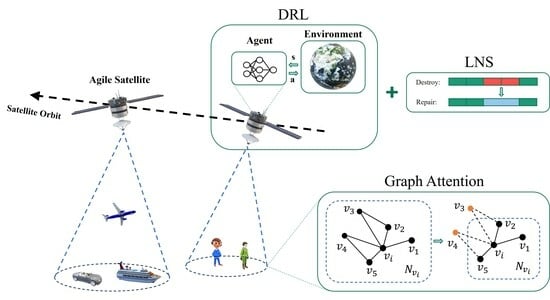
In this paper, we propose a satellite mission planning algorithm based on the dynamic destroy deep-reinforcement learning (D3RL) model, which combines the DRL framework with the LNS algorithm to enhance adaptability and computation efficiency while maintaining the quality of the solution. Specifically, a GAT-based D3RL model is designed to address the challenges of agile-satellite mission planning. First, based on the MDP, the Proximal Policy Optimization (PPO) algorithm [33] is used to train the D3RL model. Later, we integrate the DRL strategy with the heuristic algorithm and apply the D3RL model to the adaptive destruction process of the LNS. Furthermore, the DRL method, which extends the application scope of the D3RL model, also demonstrates promising outcomes.

The following is a summary of the main contributions:

• A D3RL model is designed for the AEOS scheduling problem, focusing on large-scale scenarios. The state, action, and reward function is clearly explained in MDP.
• A GAT-based actor-network is established using the target clustering information. The clustering graph for the satellite mission is built using an adjacency matrix based on the constraints provided.
• Two application methods for practical agile-satellite mission planning are proposed: the DRL method and the DRL-LNS method. The DRL method utilizes the D3RL model for direct inference, while an improved dynamic destroy operator based on the D3RL model is developed for the DRL-LNS.
• Comparison experiments are implemented between our algorithms and other algorithms (GA, ALNS). The results show that the proposed methods have fewer iteration times to convergence and a higher task-scheduled rate than other traditional heuristic algorithms in large-scale scenarios. The DRL-LNS method outperforms other algorithms in Area instances, while the DRL method performs better in World scenarios.

The remaining sections of this study are structured as follows: In Section 2, the problem description is introduced. In Section 3, the modeling process of the D3RL model is presented in depth. The effectiveness of the suggested applications are verified through comparison experiments in Section 4, and the conclusions are drawn in Section 5.

2. Problem Description

AEOS mission planning is an oversubscribed problem which requires a satellite to schedule more tasks than its capacity. As depicted in Figure 1, agile satellites with three-axis maneuvering capabilities must schedule a considerable number of remote sensing missions within a limited time frame. Based on previous research, the general objectives and constraints of the AEOS schedule problem are widely discussed in Wang et al. [7], Peng et al. [13], and Liu et al. [19]. Considering the constraints, the objective function of satellite mission planning is described as maximizing the total profit of all scheduled tasks. In this section, some problem assumptions and detailed mathematical formulations are set up for a specific scenario.

2.1. Problem Assumption

The mathematical formulation of agile-satellite mission planning in actual satellite remote sensing scenarios is highly complex due to the flexibility of satellite maneuvering, the diversity of satellite loads, and the complexity of remote sensing tasks. In this study, we focus solely on the task decision component of agile-satellite mission planning. To make this feasible, we make some reasonable simplifications and assumptions based on actual engineering backgrounds [34]:

• Each task can only be executed once, and the profit can be obtained when the task is scheduled.
• The execution time windows of any two scheduled tasks cannot overlap and must be within the visible time window.
• Satellite storage, power constraints, and image download processes are not considered. Resource problems are not the key factor for short-term mission planning [6].
• Most of the tasks are regular with equal profit.
• Only the single-orbit scenario of a single satellite is taken into account.

Remark 1.

This paper primarily addresses the normalized monitoring scenario of remote sensing satellites, where regular tasks constitute the majority of actual satellite remote sensing observation tasks, with only a small number of emergency tasks. In this context, the profit differences between regular tasks are not apparent, making the direct assignment of task priority based on profit, as some current studies do, unreasonable. To assess the efficiency of regular task planning, this paper introduces the task scheduled rate, which is defined in Section 4.3. Future research will delve into a detailed analysis of the profit function.

2.2. Variables

Define the task set: R = $\{r_1,r_2,\dots ,r_n\}$, where $r_i$ is the i-th task and n is the total number of target points. $X=\{x_1,x_2,\dots ,x_n\}$ is the n-dimensional decision vector, where $x_i\in \{0,1\}$, $i\in \{1,2,\dots ,n\}$. The task is selected to be completed when $x_i=1$. $[w_i^s,w_i^e]$ and $[t_i^s,t_i^e]$ can be calculated using the known satellite orbit and target information. Within the selected visible time window $[w_i^s,w_i^e]$, the satellite has the capability to detect targets either through maneuvers or directly within the field of view. The task-execution time window $\left[t_i^s,t_i^e\right]$ refers to the specific time during which a satellite task is executed, such as the period when an optical observation satellite takes photographs.

2.3. Mathematical Formulation

2.3.1. Constraint Conditions

• Conflict constraint:
  A satellite can only perform one mission per observation. There is no crossover between any two tasks, as the optical sensor cannot perform two observation tasks at the same time. $\forall u,v\in \{1,2,\dots ,n\}$ and $u\ne v$:

  $$[t_u^s,t_u^e]\cap [t_v^s,t_v^e]=\varnothing$$

  (1)
• Task execution uniqueness constraint:
  In this paper, we do not consider repetitive tasks. Each task can just be observed at most once in all satellite observation periods:

  $$x_i=\sum _{j=1}^{|{\mathbf{OW}}_{\mathbf{i}}|}{x}_i^j\le 1,\forall r_i\in R$$

  (2)
  ${\mathbf{OW}}_{\mathbf{i}}$ is the execution time window set for task $r_i$. We define the $x_i^j$ as a binary decision variable indicating whether the j-th excution time window of ${\mathbf{OW}}_{\mathbf{i}}$ associated with task $r_i$ is selected or not. It means that for each task we can choose only one execution time window to fulfill its observation.
• Satellite-attitude maneuver time constraint:
  The actual observation time of the task $r_u$ must be within a visual time window of the task:

  $$w_u^s\le t_u^s\le t_u^e\le w_u^e$$

  (3)

  $$t_u^e=t_u^s+t_u^d$$

  (4)
  Then, we can obtain the satellite-attitude maneuver time constraint between $r_u$ and $r_v$:

  $$t_u^e+t_{uv}^r\le t_v^s$$

  (5)
  The transition time $t_{uv}^r$, as defined in [19], is approximated using a piecewise linear function. The time interval between two scheduled tasks must exceed the transition time required for the satellite attitude maneuver. In the subsequent specific experiments, the transition time is set as in [35].

2.3.2. Optimization Objective

The specific observation time selection of the satellite is simplified, and the intermediate of the visible time window of the mission is temporarily set as the optimal observation time [19]. This is attributed to the characteristics of agile-satellite observation, where the optimal imaging quality and observation angle can be achieved through observation at the intermediate of the visible time window of the mission.

If $t_i^s$ is the dynamic selected, this introduces a joint problem involving mission planning and optimal control, which will be explored in future research. Then, the agile-satellite mission planning problem will become a constraint satisfaction integer programming problem. To maximize the total observation profit, more tasks will be scheduled. Hence, the objective function f is designed to maximize the total profit by the sum of scheduled tasks. In this paper, we only consider the equal profit task, which means $w_i=1$.

$$f=max\left(\sum _{i=1}^n\frac{x_i}{n}{w}_i\right)$$

(6)

Remark 2.

Agile-satellite mission planning can be described as a multi-objective optimization problem which needs to determine the observation time, observation order, and optimizing satellite control at the same time [36]. In this study, we focus on addressing the decision-making problem of the observation order for large-scale satellite missions.

3. Modeling Process

In this section, we provide a detailed explanation of the specific modeling process employed by the D3RL model. This encompasses the creation of the clustering graph, a description of the GAT network architecture, and the formulation of the MDP.

3.1. Clustering Graph

For intensive large-scale observation, clustering operations can effectively reduce the scale of the solution search space, decrease task conflicts, and improve problem-solving efficiency. This paper focuses on leveraging clustering information to generate the clustering graph and enhance the search speed for the optimal solution. The clustering model for the satellite mission is built using graph theory in accordance with the provided constraints [12,37]:

$$w_v^e-w_u^s\ge \mathsf{\Delta }T$$

(7)

$$|{\theta }_u-{\theta }_v|\le \mathsf{\Delta }\theta$$

(8)

Equations (7) and (8) are the detail constraints of the time window and slewing angle in the clustering process, where $\mathsf{\Delta }T$ and $\mathsf{\Delta }\theta$ are the specific observation time and angle limit thresholds, respectively. Whenever two adjacent tasks, u and v, meet the constraint conditions, the points u and v are connected by the edge $e_{uv}$.

The model consists of a graph, $G=\langle V,E\rangle$, comprising a set of vertices, V, and a set of edges, E. The vertices, $V\left(G\right)$, represent the observation tasks. The edges, $E\left(G\right)$, represent the connecting lines between points that satisfy the clustering constraints. All edges that satisfy the clustering constraints are included in $E\left(G\right)$. This way, the undirected graph model, $G=\langle V,E\rangle$, can be utilized to represent the clustering scenario of the satellite among the observable original tasks. After the embedding operation described in Section 3.3.1, the original tasks $r_1$, $r_2$, …, $r_n$ are transformed into a set of vertices $V=\{v_1,v_2,\dots ,v_n\}$ in the graph. Each vertex $v_i$ represents one task in the original task set. If a pair of vertices $(V_u,V_v)\in E\left(G\right)$, then the matrix entry $A_{uv}$ is assigned a value of 1; otherwise, $A_{uv}$ is set to 0. Below are the steps to construct the task cluster graph:

• Iterate through all tasks in $V\left(G\right)$ and construct an $n\times n$ adjacency matrix A initialized with zeros. If the two original tasks u and v satisfy the time window constraint, set $A_{uv}$ to one. This process generates the edge, $(V_u,V_v)$, and eventually constructs the graph $G_1$.
• Examine each edge in $G_1$ and remove it if its two endpoints do not meet the roll angle constraint. This results in a task clustering graph $G_2$.
• The clustering algorithm concludes, yielding the final clustering graph G and its corresponding $n\times n$ adjacency matrix A.

3.2. GAT-Based Network

3.2.1. Graph Attention Layer

The clustering graph is described as a large-scale sparse matrix. The neighboring nodes typically possess two characteristics: geographical proximity and alignment within a satellite’s visual strip, which are determined using the observation mode of satellites. GAT serves as an effective approach for processing clustering graph data. In comparison with GCN, GAT offers higher computational efficiency and enables dynamic adjustment of node importance weights. As shown in Figure 2, each graph attention layer consists of the attention and the aggregation operations [38]. Task features have been embedded based on the clustering graph $G=\langle V,E\rangle$. The input to our layer is a set of graph nodes $V=\{v_1,v_2,\dots ,v_n\}$, $v_i\in {\mathbb{R}}^F$, where n is the number of nodes and F is the number of features in each node; it is described in Section 3.3.1. After the processing of the graph attention layer, we can obtain an output vector $V^{\prime }=\{v_1^{\prime },v_2^{\prime },\dots ,v_n^{\prime }\}$, $v_i^{\prime }\in {\mathbb{R}}^{F^{\prime }}$.

In the attention operation, a weight matrix, $W\in {\mathbb{R}}^{F^{\prime }\times F}$, is first performed on the input. Then, we can calculate the attention parameter:

$${\alpha }_{\mathrm{ij}}=\frac{exp\left(\mathbf{LeakyReLU}\left(a^T[W{v}_i\Vert W{v}_j]\right)\right)}{{\sum }_{v_k\in N_{v_i}}exp\left(\mathbf{LeakyReLU}\left(a^T[W{v}_i\Vert W{v}_k]\right)\right)}$$

(9)

where ‖ represents the concatenation operation and ${(·)}^T$ represents the transpose of a vector, $N_{v_i}$ is the one-hop neighborhood of node $v_i$, a is the map** vector, and LeakyReLU is a nonlinear activation.

The purpose of the aggregation operation is to aggregate the embedding vector according to the attention parameters. The multi-head attention mechanism is applied to enable node embeddings to stably represent the node $v_i$, resulting in the following output:

$$v_i^{\prime }{=\Vert }_{k=1}^K\sigma (\sum _{v_j\in N_{v_i}}{\alpha }_{ij}^k{W}^k{v}_j)$$

(10)

where the weight matrix of transformation $W^k$ and attention coefficient ${\alpha }_{ij}^k$ are computed using the k-th independent attention mechanism among a total of K mechanisms. Subsequently, a nonlinearity $\sigma$ is applied.

3.2.2. GAT-Based Actor-Network

The architecture of GAT-based actor-networks is illustrated in Figure 3. The input and output of the actor-network are described in detail in Section 3.3. To extract node features, we employ a multi-layer GAT approach. Initially, three graph attention layers are utilized to form a GAT block. For each block, the structure of GAT→GAT→GAT facilitates spatial exploration and expands the acceptance field to the current solution. Subsequently, the GAT block is repeated N times to decrease the graph’s density. The value of N is dependent on the node density of the actual graph, and a larger value can be selected for denser graphs.

A Gated Recurrent Unit (GRU) is employed to integrate information from historical solutions [39]. At each iteration, the hidden state $h_t$ helps calculate the output as a multiplicative adaptive weight in the final layer. The configuration of network layers and GRU is informed by the approach outlined in [40].

The output of the last layer in the actor-network represents the probability of removing each node, and it is obtained using a softmax function. We sampled nodes based on the normalized removal probability. The total count of selected removal action nodes M is determined according to Equation (11):

$$M=⌊n\times r^d⌋$$

(11)

In the above formula, n denotes the initial total number of task nodes, and $r^d$ is the preset destroy rate, which ranges from 0 to 1. We sampled the top M nodes with the highest removal probability to create a set of removal action nodes:

$$\mathsf{\Omega }=\{{\mathsf{\Omega }}_1,{\mathsf{\Omega }}_2,\dots ,{\mathsf{\Omega }}_M\}$$

(12)

The hidden state $h_t$ of GRU and the ELU function are utilized to generate two node coefficients, ${\beta }_i$, and ${\gamma }_i$, for each node i, which are then used to construct a sampling probability distribution $Beta({\beta }_i,{\gamma }_i)$. The corresponding removing coefficients were sampled from $Beta({\beta }_i,{\gamma }_i)$ for each removing action node:

$$\mathsf{\Lambda }=\{{\mathsf{\Lambda }}_1,{\mathsf{\Lambda }}_2,\dots ,{\mathsf{\Lambda }}_M\}$$

(13)

The concept of $\mathsf{\Omega }$ and $\mathsf{\Lambda }$ constitute two essential parameters in the “destroy” process, and their specific usage is elaborated on in Section 3.3.2.

3.3. Markov Decision Process Modeling

The interaction between agent and environment is depicted in Figure 4. Firstly, the state vector is embedded based on the clustering graph discussed in Section 3.1. Subsequently, the embedded initial state is fed into the actor-network to obtain the destroy nodes and the coefficients of destroy range of the current solution. Once the environment receives an action from the agent, a new state and the corresponding reward of this action are calculated. The agent repeatedly outputs actions until the terminal state is reached. The state, action, and reward of the MDP are introduced in this section.

3.3.1. State Space

In order to facilitate the extraction of node features by the graph neural network, the task information ($t^d,t^s,t^e,Roll,Pitch$) and environmental information (P, T) are embedded into a seven-dimensional vector, as shown in the input and embedding of Figure 3:

$$s_i=\left[t_i^d,t_i^s,t_i^e,Rol{l}_i,Pitc{h}_i,P_i,T_i\right]$$

(14)

where, in Equation (14), the first three dimensions, $t^d$, $t^s$, and $t^e$, are defined in

Table 1. Summary of variables and notation.

Name	Description
$r_i$	The i-th task
$x_i$	A binary variable representing whether task $r_i$ is selected
$[w_i^s,w_i^e]$	The selected visible time window for task $r_i$
$[t_i^s,t_i^e]$	The selected execution time window for task $r_i$, which is a subset of ${\mathbf{OW}}_{\mathbf{i}}$
$t_i^d$	Execution time for task $r_i$
$w_i$	The profit for task $r_i$
$t_{ij}^r$	Satellite attitude maneuver time between tasks $r_i$ and $r_j$
${\theta }_i$	Satellite observation angle for task $r_i$
${\mathbf{OW}}_{\mathbf{i}}$	The set of task-execution time windows for task $r_i$
$v_i$	The i-th embedded graph node
W	The weight matrix of transformation
$Rol{l}_i$	Roll attitude angle observed by the satellite to the task node i
$Pitc{h}_i$	Pitch attitude angle observed by the satellite to the task node i
$S_t$	The state in t-th iteration
$A_t$	The action in t-th iteration
$\mathsf{\Omega }$	The set of removing action nodes
$\mathsf{\Lambda }$	The set of corresponding removing coefficients
$G_t$	The reward function
R	The discounted cumulative reward

, representing the task-execution time, task-start execution time, and task-end execution time. $Rol{l}_i$ and $Pitc{h}_i$ represent the roll and pitch attitude angles observed by the satellite to the task node i, respectively [35]. $s_i^t$ denotes the embedded vector in the t-th iteration, while $P_i$ and $T_i$ represent the cumulative profit and execution time, respectively, of the scheduled list corresponding to the t-th iteration. $t^d$, $Roll$, and $Pitch$ are normalized by the corresponding maximum value in the task node; $t^s$ and $t^e$ are normalized by the total planning time; and P and T are normalized by the total cumulative value of the scheduling process.

Therefore, the state space is defined as a vector containing task information, scheduled task lists, and environmental information:

$$S_t={[s_1^t,s_2^t,\dots ,s_n^t]}^T$$

(15)

$S_t$ represents the current state in the t-th iteration. As shown in Equation (15) and Figure 3, each element of $S_t$ represents a scheduled embedding task vector $s_i^t$.

3.3.2. Action Space

The actor-network will generate action destroy nodes $\mathsf{\Omega }$ and destroy coefficients $\mathsf{\Lambda }$. Then, the tasks will be rescheduled when the removeing nodes are calculated according to action destroy nodes and the coefficients. The architecture of the actor-network is depicted in Figure 3. Graph feature extraction was conducted using a multi-layer GAT network. Specific network parameters refer to [40].

$$A_t=({\mathsf{\Omega }}^t,{\mathsf{\Lambda }}^t)$$

(16)

In the t-th iteration, $A_t$ represents the action, ${\mathsf{\Omega }}^t$ represents the removing action nodes, and ${\mathsf{\Lambda }}^t$ is the corresponding removing coefficients.

For the n-dimensional decision vector in the t-th iteration, $X_t=\{x_1^t,x_2^t,\dots ,x_n^t\}$. If the scheduled embedding task vector $s_i^t$ is removed from $S_{t-1}$, the corresponding value $x_i^t$ will be set to 0.

According to the defined state and action space, the state transitions with a given action by adhering to the dynamic process:

• Initialize all the parameters, given a feasible initial decision vector $X_t$ and state $S_t$.
• “Destroy” process: We determined the final set of removal points $RemovingNode{s}_t$ using ${\mathsf{\Omega }}^t$ and ${\mathsf{\Lambda }}^t$. The length of the removal point set, denoted as $M^{\prime }$, is also influenced by the predetermined destroy rate $r^{d^{\prime }}$. Similar to Equation (11), the computation process is as follows:

  $$M^{\prime }=⌊\frac{n\times r^{d^{\prime }}}{M}⌋\times M$$

  (17)

  where both n and M are defined in Equation (11). Taking the example of destroy action node ${\mathsf{\Omega }}_i^t$, we performed sampling among its neighboring nodes (including the ${\mathsf{\Omega }}_i^t$). The sampling space is defined as the set of $NeighborNode{s}_i$, with the sampling rate set to ${\mathsf{\Lambda }}_i^t$, and the number of sampled points set to the product of $|NeighborNode{s}_i|$ and ${\mathsf{\Lambda }}_i^t$. The $RemovingNode{s}_t$ is generated by sampling $M^{\prime }$ points from the entire set of destroy points. According to the $RemovingNode{s}_t$, the corresponding value of $X_t$ is set to 0, and the corresponding nodes are removed in $S_t$.
• “Repair” process: The repair process involves re-planning, where the repair operator TimeInsert is employed to include task nodes that adhere to the constraints in $S_t$, setting the corresponding decision variables in $X_t$ to one, thereby generating a new state $S_{t+1}$. TimeInsert, which is a designed repair operator, will improve the destroyed solution by inserting new tasks into it, following the time sequence of the task’s arrival [19].

3.3.3. Reward

Designing a better reward function can expedite the convergence of the model training process. In this study, we evaluate the efficiency of the dynamic destroy operator by considering the total profit of the scheduled tasks, denoted as f, as defined in Equation (6).

$$\begin{array}{cc}\hfill G_t& =f\left(TimeInsert\left(X_t\right)\right)-f\left(TimeInsert\left(X_{t-1}\right)\right)\hfill \\ \hfill R& =\{G_1,G_2,\dots ,G_t,\dots \}\hfill \end{array}$$

(18)

where R is the discounted cumulative reward, and the reward function $G_t$ is set as the difference in the total profit.

3.3.4. Training Process

The model was trained using the PPO algorithm framework [33], which is easily tuned and easy to implement. The loss function of PPO is defined as [40]:

$$\begin{array}{cc}\hfill L^{clip}\left(\theta \right)& =E_t\left[min(r_t\left(\theta \right)ad{v}_t,clip(r_t\left(\theta \right),1-{ϵ}_{clip},1+{ϵ}_{clip})ad{v}_t)\right]\hfill \\ \hfill L^{vf}\left(\theta \right)& =MSE({\varphi }_{\theta }\left(S_t\right),R)\hfill \\ \hfill L_t\left(\theta \right)& =E_t[L_i^{clip}\left(\theta \right)-c_1\ast L_t^{vf}\left(\theta \right)+c_2\ast S\left[{\pi }_{\theta }\right]\left(S_t\right)]\hfill \end{array}$$

(19)

where $ad{v}_t$ is the advantage function, $r_t\left(\theta \right)=\frac{{\pi }_{\theta }\left(A_t\right|S_t)}{{{\pi }_{\theta }}_{old}\left(A_t\right|S_t)}$ denotes the probability ratio, and ${\varphi }_{\theta }\left(S_t\right)$ is the state-value function. R is the discounted cumulative reward. $c_1$ and $c_2$ are hyperparameters and $S\left[{\pi }_{\theta }\right]$ is an entropy bonus of ${\pi }_{\theta }$. The critic network is built by the form of three fully connected layers, whose input is the hidden state $h_t$ of the actor-network. The training process is illustrated in Algorithm 1.

Algorithm 1 Training process based on PPO

Input:  Tasks list Output:  The new mission planned index list   1: Initialize policy params $\theta$   2: for scene in training Scenarios do   3:     Import a new scene   4:     for Iteration = 1, 2, …, I do   5:         Parameters initialization   6:         for t = 1, 2, …, $t_m$ do   7:            Get action $A_t$ from policy ${\theta }_{old}$   8:            Update new state $S_{t+1}$   9:            Calculate instant reward $R_t$ 10:            Put $[S_t,A_t,R_t,S_{t+1}]$ into memory buffer B 11:            Calculate advantage estimates $ad{v}_1$, $ad{v}_2$, …, $ad{v}_{t_m}$ 12:         end for 13:         for epoch = 1, 2, …, K do 14:            Sample a random minibatch of N transitions $[S_t,A_t,R_t,S_{t+1}]$ from B 15:            Computing training loss as in (19) 16:            Update $\theta$ with stochastic gradient ascent 17:            ${\theta }_{old}\leftarrow \theta$ 18:         end for 19:     end for 20: end for

3.4. Applications

The trained D3RL model focuses on the destroy process of the existing solution and needs to be complemented with a repair process to obtain a viable solution for agile-satellite mission planning. To address this, we designed two applications of the D3RL model: the DRL method and the DRL-LNS method. The DRL method utilizes the D3RL model for inference directly, then use the TimeInsert operator to repair and obtain a feasible solution. In the DRL-LNS method, we integrated the D3RL model as a dynamic destroy operator within the LNS framework, which finds the local optimal solution via heuristic iteration. The specific steps of the DRL-LNS approach are shown in Algorithm 2.

Algorithm 2 DRL-LNS

Input:  Testing Scenarios Output:  $Average\left(X\right)$   1: for scene in Testing Scenarios do   2:     Import test Scenario   3:     Initial dynamic removal, repair operators D, $Random$   4:     Initial solution: $x=Initial\left(x_0\right)$   5:     repeat   6:         $x^i=Random\left(D\left(x\right)\right)$   7:         if accept $x^i$ then   8:            $x=x^i$   9:         end if 10:         if $f\left(x^i\right)<f\left(x^{*}\right)$ then 11:            $x^{*}=x^i$ 12:         end if 13:     until Terminal condition is met 14:     Put $x^{*}$ into X 15: end for

Remark 3.

The implementation of the DRL-LNS algorithm can be divided into four steps:

1.

Parameter initialization. The initial solution, denoted as $x_0$, can be arbitrary. The initialization function, $Initial$, checks the initial solution for compliance with the rules and reorders it according to the constraints to obtain a feasible initial solution.

2.

Destruction and repair process. Tasks are first removed from the current solution, and then new tasks are added to generate a new solution. The repair process employs a $Random$ repair operator, which randomly samples from the set of pending tasks when inserting new tasks. The destruction process utilizes the D3RL-based destruction operator, denoted as D.

3.

Parameter update. The obtained solution is evaluated, and if the reward of the new current solution improves, parameter updates are performed. We mainly use simulated annealing for optimal solution selection.

4.

Termination criterion determination. If the termination criterion is met, the algorithm ends and returns to the optimal value. If not, the iteration continues to search for solutions.

4. Experimental Simulation

4.1. Simulation Scenarios

We obtained the original AEOS mission targets dataset from [35]. As shown in

Table 2. Simulation scenarios.

Scenario	Region	Num of Points	Instance Sizes	Training Scenarios	Test Scenarios
Area	3°N–53°N, 74°E–133°E	400	50, 100, 150, 200	20	10
World	65°S–65°N, 180°W–180°E	600	100, 200, 300, 400	20	10

, the targets were generated over two geographical regions: Area and World. Area targets are defined by the area corresponding to 3°N–53°N and 74°E–133°E, and the World targets are located randomly in a region of 65°S–65°N and 180°W–180°E. Regarding the observed target data, there is currently no reliable publicly available real dataset. It is worth noting that the majority of the literature also uses simulated generated targets, often employing random generation. Maintaining generality, we have aligned the simulation scenarios with theirs [18,19,30,31].

The existing 1000 original point targets (Area: 400, World: 600) were sampled multiple times and divided into different scenarios of various sizes. A total of 50 to 200 Area tasks and 100 to 400 World tasks were sampled to simulate practical users’ requests. We sampled randomly to generate 20 training scenarios and 10 test scenarios for each instance size.

4.1.1. Task Scheduled Rate

In scenarios involving intensive regular tasks, the primary evaluation metric for planning is the number of scheduled tasks. Given that there is no significant difference in the profit of regular tasks, the task scheduled rate serves as a more accurate reflection of the algorithms’ planning efficiency. Emergency tasks, on the other hand, can be given priority and scheduled in advance to ensure their timely execution. The calculation formula of the task scheduled rate is as follows:

$$r_s=\frac{n_{Scheduled}}{N_{Total}}$$

(20)

where $n_{Scheduled}$ is the number of tasks that have been scheduled, and $N_{total}$ is the total number of tasks waiting for planning.

4.1.2. Algorithm Parameters

We chose a task at random to serve as the initial solution first, fixed it using the TimeInsert repair operator, and then derived the repaired solution, which was organized chronologically. All experiments were implemented by Pytorch in Python and compared on a computer with Intel Core i5-12500H CPU @ 4.50 GHz, 16 GB RAM. Parameters of the training model are shown in

Table 3. Training parameters.

Parameters	Value
Learning rate	0.001
Discount factor $\gamma$	0.99
The clip rate ${ϵ}_{clip}$	0.2
Batch size	16
Number of iterations in each scene	3000
Number of training scenes	20
Number of epoch K	2
Destroy rate	0.2
Initial temperature	100
Final temperature	1

.

4.2. Training Performance

Training Comparison

The training process of D3RL model is essentially similar to solving a local optimal solution using the heuristic algorithm [20,22]. Each iteration is a dynamic destruction of the existing local optimal solution, and the TimeInsert operator is used for a repair.

Figure 5 illustrates that the agent can continue to achieve an improved task scheduling rate as the number of iterations increases, and with sufficient iterations, the training process converges. In Figure 5a, the scheduled rate gradually decreases as the number of tasks in the intensive $Area$ scenario increases. The convergence of each scenario is influenced by the specific difficulty of task planning, which is the primary reason for the reduction in the scheduled rate. The more challenging the task planning, the more iterations are required for convergence, and it does not simply correlate positively with the number of targets in the region.

Figure 5b exhibits a similar trend to the $Area$ scenario. Due to the increase in the number of tasks and the expansion of the coverage area, the model for the “World” scenario generally approaches convergence after 4000 iterations, which is considerably more than the “Area” scenario. Additionally, in the seed sensitivity experiments, it was observed that the “World” scenario is much more sensitive to the random seed settings compared with the “Area” scenario, particularly for the instance with a task count of 100. This sensitivity is particularly pronounced for the instance with 100 tasks, where the planning rate notably increases for two specific random seed settings. As a result, the average task planning rate for instance 100 is considerably higher than instances with larger numbers of tasks. For subsequent validation experiments, we employed a consistent random seed across scenarios.

4.3. Testing Performance

4.3.1. Model Generalization Test

We transferred a trained model to other instances in the training dataset.

Table 4. Comparison of model generalization on train set.

Methods	Area				World
	50	100	150	200	100	200	300	400
train_50	0.5080	0.3460	0.3387	0.3070	0.6160	0.5980	0.6020	0.6215
train_500	0.5120	0.3660	0.3493	0.3230	0.6560	0.6080	0.6120	0.6280
train_5000	0.5360	0.3920	0.3827	0.3600	0.7020	0.6680	0.6667	0.6740
trained	0.5280	0.3860	0.3600	0.3310	0.6720	0.6280	0.6240	0.6470

Metric is scheduled rate.

and Figure 6 demonstrate the generalization ability of a well-trained agent in different instances of training. This is mostly attributed to the similarities of the planning tasks and the significant generalization ability of the D3RL model.

Initially, a scenario was randomly sampled from the training set for each instance size to train the scheduling network. Afterwards, the trained network was utilized to process the remaining training instances in the set (the results are denoted as $trained$). This was primarily performed to assess the model’s generalization ability. Models that perform well in unknown training scenarios demonstrate reduced reliance on specific data and require a smaller training set. The variable $train\_num$ in Table 4 represents the average training results obtained from 10 unknown scenes in the training set. The training process consisted of a specific number of iterations denoted by the variable $num$, which can take three values: 50, 500, and 5000. As shown in the training curves of Figure 5, the training process was considered to be completely convergent when iteration times exceeded 5000.

In the $Area$ data (Figure 6a), the scheduled rate obtained through model inference ($trained$) can even reach 91.9% to 98.5% of model converged ($train\_5000$). Similarly, in the $World$ instances (Figure 6b), the scheduled rate can range from 93.3% to 96%. In the $World$ instances depicted in Figure 6b, the results of direct model inference ($trained$) exhibit a similar pattern to the $Area$ instances. However, the task scheduled rate does not simply decrease as the number of tasks increases. Interestingly, when the observed targets increase from 300 to 400, the task scheduled rate actually improves. This phenomenon can be attributed to the fact that the observed targets in the $World$ instances are extremely sparse compared with the targets in the $Area$ instances. Increasing the number of observable target points can enhance the task scheduled rate in scenarios where there are relatively few target points to begin with. In the results depicted in Figure 6, for the $train\_num$ results, it is evident that as the instance size increases, the height of the boxes consistently decreases. With 50 iterations of training, the model’s training remains incomplete, resulting in a more dispersed distribution of outcomes. This corresponds to the training process. Within the $Area$ scenario results, the results of $trained$ also become more concentrated with the enlargement of the instance size. However, this characteristic is not observed within the $World$ scenario. This discrepancy could potentially be attributed to the larger geographical scope and the significant variations in the distribution of target points in the $World$ scenario.

We have conducted some ‘transfer’ experiments (i.e., trained the model on the World, then evaluated it on some Area setups) and found that the model’s generalization performance between “Area” and “World” scenarios is not satisfactory. The inference results of the well-trained model in “Area” were slightly lower than training a new model for the “World” scenario 500 times. This might be attributed to the significant differences between “Area” and “World” scenarios and the scenario dependence of our DRL model.

4.3.2. Comparison of Algorithms Test

Table 5. Comparison of the iteration times.

Scenarios	Average Scheduled Rate 1
	GA	ALNS	DRL-LNS	DRL
Area_50	0.2640	0.4680	0.5000	0.4080
Area_100	0.2400	0.3760	0.4020	0.3640
Area_150	0.2080	0.3267	0.3747	0.3107
Area_200	0.0000	0.3010	0.3520	0.2840
World_100	0.6000	0.6620	0.7000	0.7020
World_200	0.0000	0.6150	0.6400	0.6660
World_300	0.0000	0.6093	0.6320	0.6640
World_400	0.0000	0.5795	0.5940	0.6350

¹ Iteration times for GA/ALNS/DRL-LNS was 1500.

and Figure 7 present the performance of different optimization algorithms in terms of the task scheduled rate across 10 test scenarios for each instance size. The DRL application method is denoted as DRL. In the comparison of the DRL-LNS, GA [41], and ALNS [42] algorithms, the number of iteration times was set to 1500. Agile-satellite mission planning problem is NP-hard. Our goal was not to obtain the optimal solution, but rather to achieve a satisfactory feasible solution within the constrained resources and time, which differs significantly from ground-based optimization scenarios. We chose 1500 iterations as an economically viable solution, considering the trade-off between solution quality and computational cost. The specific value of 1500 iterations may vary based on the specific context. It was observed that the GA algorithm failed to find a feasible solution when the number of planning tasks exceeded 200. In contrast, the other comparison algorithms, including DRL-LNS and ALNS, successfully completed the planning process. As a result, the task scheduled rate of the GA algorithm exceeding 200 was 0.

In Figure 7a, the task scheduled rate of our DRL-LNS algorithm is, on average, 11.35% higher than those of the ALNS for $Area$ instances. With the increase in instance size, the gap between ALNS and DRL-LNS increases and becomes the highest at 200, which is around 17%. It can be found that the task scheduled rate of DRL method is slightly lower (average 6.6%) than that of ALNS algorithm, which is consistent with the results obtained by the current main neural network learning algorithm [28,30,31]. From the above results, it can be found that the combination of the GAT-based model and heuristic algorithm brings about a notable enhancement in the computational efficiency of the algorithm. This improvement is particularly prominent when dealing with large-scale complex constraint problems that involve dense targets in local regions. At the same time, due to the increase in tasks that cannot be completed in the over-intensive scenarios, the scheduled rate declines with the increase in the number of $Area$ missions.

Compared with the $Area$ scenarios, the $World$ instances involve planning more tasks, but the actual task distribution may be much sparser than the regional scope. As shown in Figure 7b, the DRL method achieved the best performance on the $World$ instances, in which the task scheduled rate of the DRL approach was, on average, 8.2% higher than those of the ALNS. In large-scale AEOS task scheduling problems, heuristic algorithms are limited by time and resource constraints and can only converge to suboptimal solutions. As the scale and complexity of the problem increase, along with tighter time and resource constraints, the quality of the solutions obtained through a heuristic search deteriorates, leaving room for improvement in solution quality for the DRL approach. Neural networks have an advantage in handling large-scale data. The use of the D3RL model enhances the algorithm’s adaptability to highly complex problems, and the GAT network allows for faster extraction of relevant features from the data. These enable the DRL method to obtain satisfactory suboptimal solutions in a single inference.

The results indicate that the D3RL-based approaches (DRL-LNS, DRL method) have faster convergence speeds and higher solution quality than the traditional heuristic algorithms (GA and ALNS). And the DRL-LNS is more suited to scenarios with regionally dense targets on a small scale (less than 200), while the DRL method is better-suited to scenarios with large-scale global targets (more than 200). Figure 8 displays a detailed comparison of the algorithm iteration curves for both $Area$ and $World$ instances.

5. Conclusions

To address the challenges of large-scale regular mission planning for agile satellites, the D3RL model based on GAT is established by using the target clustering information. Building upon the D3RL model, we propose two applications for agile-satellite regular task planning: DRL and DRL-LNS, and a design for state, action, and reward function is developed in the MDP. In comparison with the traditional heuristic method (GA, ALNS), the simulation results show that DRL-LNS with a dynamic destroy operator performs exceptionally well on large-scale dense regional remote-sensing observation tasks. In the more challenging large-scale global remote-sensing observation tasks, the DRL method outperforms the competition. The experimental results demonstrate the proposed D3RL model is very applicable and efficient for large-scale remote-sensing observation mission planning and related large-scale planning scenarios.

The proposed dynamic destroy methods, however, may not be suited for dynamic multi-agent environments. Future research will focus on the multi-satellite AEOS planning problem with dynamic task scenarios using a multi-agent DRL approach.

References

1. Singh, P.; Pandey, P.C.; Petropoulos, G.P.; Pavlides, A.; Srivastava, P.K.; Koutsias, N.; Deng, K.A.K.; Bao, Y. Hyperspectral remote sensing in precision agriculture: Present status, challenges, and future trends. In Hyperspectral Remote Sensing; Elsevier: Amsterdam, The Netherlands, 2020; pp. 121–146. [Google Scholar]
2. Zheng, Z.; Zhong, Y.; Wang, J.; Ma, A.; Zhang, L. Building damage assessment for rapid disaster response with a deep object-based semantic change detection framework: From natural disasters to man-made disasters. Remote. Sens. Environ. 2021, 265, 112636. [Google Scholar] [CrossRef]
3. De Bem, P.P.; de Carvalho Junior, O.A.; Fontes Guimarães, R.; Trancoso Gomes, R.A. Change detection of deforestation in the Brazilian Amazon using landsat data and convolutional neural networks. Remote Sens. 2020, 12, 901. [Google Scholar] [CrossRef]
4. Chen, J.; Liu, H.; Hou, J.; Yang, M.; Deng, M. Improving building change detection in VHR remote sensing imagery by combining coarse location and co-segmentation. ISPRS Int. J. Geo-Inf. 2018, 7, 213. [Google Scholar] [CrossRef]
5. Liu, R.; Kuffer, M.; Persello, C. The temporal dynamics of slums employing a CNN-based change detection approach. Remote Sens. 2019, 11, 2844. [Google Scholar] [CrossRef]
6. Peng, G.; Dewil, R.; Verbeeck, C.; Gunawan, A.; **ng, L.; Vansteenwegen, P. Agile Earth Observation Satellite Scheduling: An Orienteering Problem with Time-Dependent Profits and Travel Times. Comput. Oper. Res. 2019, 111, 84–98. [Google Scholar] [CrossRef]
7. Wang, X.; Wu, G.; **ng, L.; Pedrycz, W. Agile Earth Observation Satellite Scheduling Over 20 Years: Formulations, Methods, and Future Directions. IEEE Syst. J. 2021, 15, 3881–3892. [Google Scholar] [CrossRef]
8. Lemaître, M.; Verfaillie, G.; Jouhaud, F.; Lachiver, J.M.; Bataille, N. Selecting and Scheduling Observations of Agile Satellites. Aerosp. Sci. Technol. 2002, 6, 367–381. [Google Scholar] [CrossRef]
9. Chu, X.; Chen, Y.; **ng, L. A branch and bound algorithm for agile earth observation satellite scheduling. Discret. Dyn. Nat. Soc. 2017, 2017, 7345941. [Google Scholar] [CrossRef]
10. Beaumet, G.; Verfaillie, G.; Charmeau, M.C. Feasibility of autonomous decision making on board an agile earth-observing satellite. Comput. Intell. 2011, 27, 123–139. [Google Scholar] [CrossRef]
11. Sarkheyli, A.; Vaghei, B.G.; Bagheri, A. New tabu search heuristic in scheduling earth observation satellites. In Proceedings of the 2010 2nd International Conference on Software Technology and Engineering, San Juan, PR, USA, 3–5 October 2010; Volume 2, p. V2-199. [Google Scholar]
12. Zhao, Y.; Du, B.; Li, S. Agile Satellite Mission Planning Via Task Clustering and Double-Layer Tabu Algorithm. Comput. Model. Eng. Sci. 2020, 122, 235–257. [Google Scholar] [CrossRef]
13. Peng, G.; Song, G.; He, Y.; Yu, J.; **ang, S.; **ng, L.; Vansteenwegen, P. Solving the Agile Earth Observation Satellite Scheduling Problem with Time-Dependent Transition Times. IEEE Trans. Syst. Man Cybern. Syst. 2022, 52, 1614–1625. [Google Scholar] [CrossRef]
14. Tangpattanakul, P.; Jozefowiez, N.; Lopez, P. Multi-objective optimization for selecting and scheduling observations by agile earth observing satellites. In Proceedings of the Parallel Problem Solving from Nature-PPSN XII: 12th International Conference, Taormina, Italy, 1–5 September 2012; pp. 112–121. [Google Scholar]
15. Geng, X.; Li, J.; Yang, W.; Gong, H. Agile satellite scheduling based on hybrid coding genetic algorithm. In Proceedings of the 2016 12th World Congress on Intelligent Control and Automation (WCICA), Guilin, China, 12–15 June 2016; pp. 2727–2731. [Google Scholar]
16. Zhang, Z.; Zhang, N.; Feng, Z. Multi-satellite control resource scheduling based on ant colony optimization. Expert Syst. Appl. 2014, 41, 2816–2823. [Google Scholar] [CrossRef]
17. Shaw, P. Using constraint programming and local search methods to solve vehicle routing problems. In Proceedings of the Principles and Practice of Constraint Programming—CP98: 4th International Conference, CP98, Pisa, Italy, 26–30 October 1998; pp. 417–431. [Google Scholar]
18. Sonnerat, N.; Wang, P.; Ktena, I.; Bartunov, S.; Nair, V. Learning a large neighborhood search algorithm for mixed integer programs. ar**v 2021, ar**v:2107.10201. [Google Scholar]
19. Liu, X.; Laporte, G.; Chen, Y.; He, R. An adaptive large neighborhood search metaheuristic for agile satellite scheduling with time-dependent transition time. Comput. Oper. Res. 2017, 86, 41–53. [Google Scholar] [CrossRef]
20. Pisinger, D.; Ropke, S. Large neighborhood search. Handbook of Metaheuristics; Springer: Cham, Switzerland, 2019; pp. 99–127. [Google Scholar]
21. Mara, S.T.W.; Norcahyo, R.; Jodiawan, P.; Lusiantoro, L.; Rifai, A.P. A survey of adaptive large neighborhood search algorithms and applications. Comput. Oper. Res. 2022, 146, 105903. [Google Scholar] [CrossRef]
22. Ropke, S.; Pisinger, D. An adaptive large neighborhood search heuristic for the pickup and delivery problem with time windows. Transp. Sci. 2006, 40, 455–472. [Google Scholar] [CrossRef]
23. Pisinger, D.; Ropke, S. A general heuristic for vehicle routing problems. Comput. Oper. Res. 2007, 34, 2403–2435. [Google Scholar] [CrossRef]
24. Hottung, A.; Tierney, K. Neural large neighborhood search for the capacitated vehicle routing problem. ar**v 2019, ar**v:1911.09539. [Google Scholar]
25. da Costa, P.; Rhuggenaath, J.; Zhang, Y.; Akcay, A.; Kaymak, U. Learning 2-opt heuristics for routing problems via deep reinforcement learning. SN Comput. Sci. 2021, 2, 1–16. [Google Scholar] [CrossRef]
26. Wu, G.; Wang, H.; Li, H.; Pedrycz, W.; Qiu, D.; Ma, M.; Liu, J. An adaptive Simulated Annealing-based satellite observation scheduling method combined with a dynamic task clustering strategy. ar**v 2014, ar**v:1401.6098. [Google Scholar]
27. Bello, I.; Pham, H.; Le, Q.V.; Norouzi, M.; Bengio, S. Neural combinatorial optimization with reinforcement learning. ar**v 2016, ar**v:1611.09940. [Google Scholar]
28. Wang, H.; Yang, Z.; Zhou, W.; Li, D. Online Scheduling of Image Satellites Based on Neural Networks and Deep Reinforcement Learning. Chin. J. Aeronaut. 2019, 32, 1011–1019. [Google Scholar] [CrossRef]
29. Chen, M.; Chen, Y.; Chen, Y.; Qi, W. Deep Reinforcement Learning for Agile Satellite Scheduling Problem. In Proceedings of the 2019 IEEE Symposium Series on Computational Intelligence (SSCI), **amen, China, 6–9 December 2019; pp. 126–132. [Google Scholar] [CrossRef]
30. Huang, Y.; Mu, Z.; Wu, S.; Cui, B.; Duan, Y. Revising the Observation Satellite Scheduling Problem Based on Deep Reinforcement Learning. Remote Sens. 2021, 13, 2377. [Google Scholar] [CrossRef]
31. He, Y.; **ng, L.; Chen, Y.; Pedrycz, W.; Wang, L.; Wu, G. A Generic Markov Decision Process Model and Reinforcement Learning Method for Scheduling Agile Earth Observation Satellites. IEEE Trans. Syst. Man Cybern. Syst. 2022, 52, 1463–1474. [Google Scholar] [CrossRef]
32. Zhang, C.; Vinyals, O.; Munos, R.; Bengio, S. A study on overfitting in deep reinforcement learning. ar**v 2018, ar**v:1804.06893. [Google Scholar]
33. Schulman, J.; Wolski, F.; Dhariwal, P.; Radford, A.; Klimov, O. Proximal policy optimization algorithms. ar**v 2017, ar**v:1707.06347. [Google Scholar]
34. Iacopino, C.; Harrison, S.; Brewer, A. Mission planning systems for commercial small-sat earth observation constellations. In Proceedings of the 9th International Workshop on Planning and Scheduling for Space (IWPSS), VenueBuenos Aires, Argentina, 25–27 June 2015; pp. 45–52. [Google Scholar]
35. He, L.; de Weerdt, M.; Yorke-Smith, N. Time/sequence-dependent scheduling: The design and evaluation of a general purpose tabu-based adaptive large neighbourhood search algorithm. J. Intell. Manuf. 2020, 31, 1051–1078. [Google Scholar] [CrossRef]
36. Wei, L.; Chen, Y.; Chen, M.; Chen, Y. Deep reinforcement learning and parameter transfer based approach for the multi-objective agile earth observation satellite scheduling problem. Appl. Soft Comput. 2021, 110, 107607. [Google Scholar] [CrossRef]
37. Wu, G.; Liu, J.; Ma, M.; Qiu, D. A two-phase scheduling method with the consideration of task clustering for earth observing satellites. Comput. Oper. Res. 2013, 40, 1884–1894. [Google Scholar] [CrossRef]
38. Veličković, P.; Cucurull, G.; Casanova, A.; Romero, A.; Lio, P.; Bengio, Y. Graph attention networks. ar**v 2017, ar**v:1710.10903. [Google Scholar]
39. Chung, J.; Gulcehre, C.; Cho, K.; Bengio, Y. Empirical evaluation of gated recurrent neural networks on sequence modeling. ar**v 2014, ar**v:1412.3555. [Google Scholar]
40. Chen, M.; Gao, L.; Chen, Q.; Liu, Z. Dynamic Partial Removal: A Neural Network Heuristic for Large Neighborhood Search. ar**v 2020, ar**v:2005.09330. [Google Scholar]
41. Jazzbin, J. Geatpy: The Genetic and Evolutionary Algorithm Toolbox with High Performance in Python. Available online: http://www.geatpy.com/ (accessed on 31 July 2020).
42. Wouda, N.A.; Lan, L. ALNS: A Python implementation of the adaptive large neighbourhood search metaheuristic. J. Open Source Softw. 2023, 8, 5028. [Google Scholar] [CrossRef]
Figure 1. Agile satellite observation. Agile satellites with three-axis maneuvering capabilities must schedule a considerable number of remote sensing missions within a limited time frame. Targets beyond the observation range remain undetectable and are therefore considered invalid.
Remotesensing 15 04503 g001
Figure 2. The process of attention and aggregation operation in graph attention layer.
Remotesensing 15 04503 g002
Figure 3. Actor-network. The attention mechanism is incorporated into the network architecture, where the initial input tasks are embedded as graph nodes. These graph nodes undergo multiple layers of GAT networks to extract node features, ultimately obtaining the set of nodes to be destroyed in the next iteration.
Remotesensing 15 04503 g003
Figure 4. Agent–environment interaction in AEOS.
Remotesensing 15 04503 g004
Figure 5. Training curves for the Area and World scenarios. The two plots show the average scheduled rate of Area and World instances, respectively. The results were obtained by conducting experiments with 5 different random seeds. (a) Training process for Area targets. (b) Training process for World targets.
Remotesensing 15 04503 g005
Figure 6. Optimization scheduled rate performance contrast. Boxplot illustrating comparison based on 10 different instances. Each box represents the interquartile range (IQR) of the data distribution, with the median marked by a horizontal line inside the box. Triangle markers indicate the mean values of the test results. (a) Scene: Area. (b) Scene: World.
Remotesensing 15 04503 g006
Figure 7. Optimization Scheduled rate performance contrast. (a) Scene: Area. (b) Scene: World.
Remotesensing 15 04503 g007
Figure 8. Performance comparison of algorithms with 1500 iterations. Each instance size evaluated across 10 test scenarios. Note: The GA algorithm fails to find a feasible solution when the number of planning tasks exceeds 200. (a) Scene: Area instance size: 50. (b) Scene: Area instance size: 100. (c) Scene: Area instance size: 150. (d) Scene: Area instance size: 200. (e) Scene: World instance size: 100. (f) Scene: World instance size: 200. (g) Scene: World instance size: 300. (h) Scene: World instance size: 400.
Remotesensing 15 04503 g008aRemotesensing 15 04503 g008b