Technical Note

Strong-Scattering Multiparameter Reconstruction Based on Elastic Direct Envelope Inversion and Full-Waveform Inversion with Anisotropic Total Variation Constraint

1
College of Geo-Exploration Science and Technology, Jilin University, Changchun 130026, China
2
Modeling and Imaging Laboratory, Department of Earth and Planetary Sciences, University of California, Santa Cruz, CA 95064, USA
*
Author to whom correspondence should be addressed.
Remote Sens. 2023, 15(3), 746; https://doi.org/10.3390/rs15030746
Submission received: 27 November 2022 / Revised: 29 December 2022 / Accepted: 25 January 2023 / Published: 27 January 2023
(This article belongs to the Special Issue Geophysical Data Processing in Remote Sensing Imagery)

Abstract

:
Strong-scattering medium can usually form a good sealing medium for oil and gas resources. However, conventional elastic full-waveform inversion (EFWI) methods are difficult to build reliable velocity models under the condition of lacking low-frequency information. The elastic direct envelope inversion (EDEI) method has been proven to be able to model large-scale Vp and Vs structures of strong-scattering media. The successive use of EDEI and EFWI can obtain fine structures of the strong scatterers and their shielding areas. However, the inversion effects of inner velocity and bottom boundaries of strong scatterers by the existing methods need to be improved. In this paper, we propose the elastic direct envelope inversion with anisotropic total variation constraint (EDEI-ATV). The anisotropic total variation (ATV) constraint has the advantage of making the velocity more uniform inside the layer and sharper on boundaries, which can be used to improve the inversion results of EDEI. During the iterations, the ATV constraint is directly applied to the update of Vp and Vs, and the alternately iterative algorithm can achieve good results. After obtaining reliable large-scale Vp and Vs structures, the EFWI with anisotropic total variation constraint (EFWI-ATV) is performed to obtain high-precision Vp and Vs structures. Numerical examples verify the effectiveness of the proposed method.

Graphical Abstract

1. Introduction

Full-waveform inversion (FWI) constructs subsurface parameter models by matching the full-waveform information of simulated data and observed data [1,2]. The sensitivity kernel of the FWI can be simplified by using the Born approximation, so that the gradient of FWI can be easily calculated by the adjoint-state method. In the absence of low-frequency information, it is difficult for the traditional FWI method to model the velocity of strong-scattering media. When multi-wave and multi-component cases are considered, the nonlinearity of elastic full-waveform inversion (EFWI) is stronger, and it is more difficult to model high-precision velocity in elastic strong-scattering media [3]. Strong-scattering media can usually form good storage media for oil and gas resources. Therefore, it is of great practical significance to build high-precision Vp and Vs models for elastic strong-scattering media.
In order to improve the velocity inversion of strong-scattering media, a series of improved algorithms for FWI method have been proposed, such as the Laplace–Fourier domain-waveform inversion method [4,5], the level set method [6], multi-dominant frequency inversion method [7], deep learning method [8], edge-preserving smoothing algorithm [9], compressed sensing and sparse constraint method [10], etc. The total variation (TV) constraint has shown advantages in the FWI, which can make the velocity inside the layer more uniform and the boundary sharper [11,12,13,14,15,16,17]. Taking this advantage, the TV constraint can play an important auxiliary role in parameter modeling of strong-scattering media. Esser et al. applied the isotropic total variation (ITV) constraint (L2 norm total variation constraint) in the acoustic adaptive-waveform inversion method, which successfully improves the accuracy and resolution of strong-scattering salt dome modeling [18]. Then, the hinge-loss strategy is introduced into the FWI with the ITV constraint, which further improves the accuracy of salt dome and sub-salt velocity modeling [19]. Qiu et al. proposed a FWI process based on steerable variation regularization, which simultaneously uses anisotropic total variational (ATV) constraint (L1 norm total variational constraint) and model space variation prior information as regularization items [20]. Peters and Herrmann [21] pointed out that applying the TV regularization constraint to the misfit function of FWI as a penalty function will cause the inversion result to become a function of smoothness and compromise parameters. They proposed to apply the intersection of the ITV and bound constraint on FWI. Yong et al. [22] proposed an adaptive primal–dual hybrid gradient method to solve the waveform inversion problem with the ITV constraint. The convergence rate and computational efficiency of this method are improved compared with the primal–dual hybrid gradient method. Kalita et al. [23] use the TV constraint FWI and an automated salt flooding strategy to obtain high-precision salt model building with the lowest available frequency of 3Hz and a simple initial model. Most of the above strong-scattering velocity modeling with TV constraint research studies are based on the acoustic media. In this paper, the ATV constraint is used for the multiparameter model building of elastic strong-scattering media.
The envelope data contains abundant ultra-low frequency information even if the original seismic data lacks effective low-frequency information. Wu et al. proposed the modulation-convolution signal model and the envelope inversion method [24,25] to recover the large-scale structures of the subsurface media. According to the modulation-convolution signal model, even if the source and seismic data lack low-frequency information, the seismic envelope data still carry the intrinsic long-wavelength scattering response of the subsurface medium. However, due to the chain rule used in deriving the gradient, conventional envelope inversion [24,26,27] cannot solve the inversion problem of large-scale strong-scattering media. In order to overcome the problems of conventional envelope inversion, Wu and Chen proposed the direct envelope Fréchet derivative and the direct envelope inversion (DEI) method [28,29,30], which directly maps the ultra-low frequency envelope data perturbation to the velocity perturbation and can invert the large-scale strong-scattering velocity model without original low-frequency information. Chen et al. [31] combined the DEI method with the wavefield direction decomposition method, and proposed a reflection DEI method, which can improve the inversion effects of the velocity structures in the strong-scattering shielding area. Chen et al. [32] and Wang et al. [33] found that the envelope data based on Hilbert transform loses polarity information, and considering polarity information in the process of DEI can improve the reconstruction of the salt domes and subsalt structures. Chen et al. [34] further explored the physical meaning of the signed envelope, pointed out its connection with the subsurface reflection coefficient sequence, and proposed a multi-scale signed DEI method. Zhang et al. [35] proposed a source-independent direct envelope inversion method, which effectively alleviates the influence of source wavelet errors on the inversion results. Chen et al. [36] combined the objective function of FWI and DEI and used the multi-offset inversion strategy to improve the inversion effect of the DEI method for the strong-scattering salt dome model. Hu et al. [37] constructed DEI in the time-frequency domain using the instantaneous amplitude and phase, which effectively improved the inversion effect of strong-scattering salt domes and sub-salt structures. Luo et al. [38] proposed an angle-domain DEI method according to the radiation pattern difference in the velocity and density, and realized the simultaneous inversion of the strong-scattering velocity and density based on acoustic media. Zhang et al. [39] introduced wavefield direction decomposition and structure-guided perturbation decomposition strategy in the process of DEI, which improves the inversion effects of salt dome and sub-salt structures. The latest studies have extended the DEI method to elastic media, which can simultaneously provide reliable large-scale Vp and Vs structures of strong-scattering media [40,41,42]. However, it is difficult for the existing DEI methods to obtain the ideal uniform velocity inside the elastic strong scatterers. The modeling effect of the bottom boundary of strong scatterers is also not ideal. Therefore, we propose to introduce the anisotropic total variational constraint into the elastic direct envelope inversion (EDEI) method.
In this paper, ATV constraint is applied in the process of EDEI, which can improve the modeling effects of the inner velocity and bottom boundaries of strong scatterers. After the reliable long-wavelength Vp and Vs structures are obtained, the EFWI with anisotropic total variation constraint can obtain high-accuracy Vp and Vs structures of the strong-scattering media. Finally, the proposed method is verified on the modified SEG/EAGE (Society of Exploration Geophysicists/European Association of Geoscientists&Engineers) salt dome model.

2. Review of Elastic Full-Waveform Inversion and Direct Envelope Inversion

2.1. Elastic Full-Waveform Inversion (EFWI)

The EFWI method conducts high-precision multiparameter model building by matching the multi-component simulated and observed data. The objective function of EFWI is
σ E F W I = 1 2 s i n s r i n r c u r i , s i c d r i , s i c 2 ,
where n s and n r denote the total source and receiver number, respectively; s i and r i denote the source and receiver index, respectively; c denotes the direction index of the recordings and c = x , y , z ; u and d denote synthetic data and observed data, respectively. According to the adjoint-state method and the chain rule, the gradient of σ E F W I with respect to P-wave velocity v p and S-wave velocity v s in 2D case can be written as [43]
σ E F W I v p = 2 ρ v p 0 T ( u x x + u z z ) ( u x + x + u z + z ) d t ,
σ E F W I v s = 4 ρ v s 0 T ( u x x + u z z ) ( u x + x + u z + z ) d t 2 ρ v s 0 T [ 2 ( u x x u x + x + u z z u z + z ) + ( u z x + u x z ) ( u z + x + u x + z ) ] d t ,
where ρ denotes density; u x and u z denote x- and z-components of the forward-propagated source wavefield, respectively; u x + and u z + denote the x- and z-component of the back-propagated residual wavefield, respectively. Due to the consideration of multiparameter inversion, EFWI is more nonlinear than acoustic FWI. It is obviously more difficult to carry out high-precision multiparameter modeling of elastic strong-scattering medium than single parameter modeling.

2.2. Elastic Direct Envelope Inversion (EDEI)

The EDEI method can reconstruct large-scale strong-scattering velocity models in the absence of original low-frequency information. The objective function of EDEI can be written as
σ E D E I = 1 2 s i n s r i n r c e r i , s i s y n , c e r i , s i o b s , c 2 ,
where e s y n and e o b s denote the envelope of simulated and observed data, respectively. In conventional envelope inversion, the gradient is calculated using the chain rule. The envelope data perturbation is firstly mapped to the data perturbation and then mapped to the velocity perturbation. The low-frequency advantages of the envelope data are weakened a lot during this process. With direct envelope inversion, the envelope data perturbation is directly mapped to velocity perturbation, so that we can handle large-scale and strong-scattering velocity perturbation [35]. In EDEI, the gradient of the objective function shown in Equation (4) with respect to v p and v s can be calculated by means of wave mode decomposition, which can be written as [37]
σ E D E I v p = 2 ρ v p s i n s r i n r 0 T E s y n p [ G e T ( Δ E ) ] p d t ,
σ E D E I v s 2 ρ v s s i n s r i n r 0 T { E s y n s , x [ G e T ( Δ E ) ] s , x + E s y n s , z [ G e T ( Δ E ) ] s , z } / μ 2 d t ,
where E s y n p denotes forward-propagated P-wave envelope field; Δ E denotes envelope data residual; [ ] p denotes decomposed P-wave component; G e T denotes transpose operator of envelope Green’s function; E s y n s , x and E s y n s , z denote x- and z-component of forward-propagated S-wave envelope-field, respectively; [ ] s , x and [ ] s , z denote x- and z-component of decomposed S-wave envelope-field, respectively. We can see from Equations (5) and (6), with wave mode decomposition, the Vp update mainly comes from P-wave perturbations and Vs update mainly comes from S-wave perturbations. This approximation ignores the contributions of the converted waves but can still give useful information of strong-scattering salt bodies. Many approximations are involved in the derivation of the EDEI method, and the inversion of large-scale strong scatterers is also difficult to obtain ideal uniform information (such as uniform velocity inside the salt body). Therefore, we consider the imposition of the ATV constraint in the EDEI process to improve the inversion stability and effects on the interior and boundaries of strong scatterers.

3. EDEI with Anisotropic Total Variation Constraint (EDEI-ATV)

3.1. Anisotropic Total Variation (ATV) Constraint

The TV constraint is one of the commonly used regularization terms in seismic FWI. Since the advantage of the TV constraint is to sharpen the image boundary and smooth the interior of the image, it is very suitable for making the boundary of the velocity model clearer and the velocity inside the salt dome more uniform during the inversion process. According to the form of the TV constraints, it can be divided into isotropic total variation (ITV) and anisotropic total variation (ATV) constraint, and the expressions are as follows
v I T V = i = 1 n z 1 j = 1 n x 1 ( v i , j v i + 1 , j ) 2 + ( v i , j v i , j + 1 ) 2 + i = 1 n z 1 | v i , n x v i + 1 , n x | + j = 1 n x 1 | v n z , j v n z , j + 1 | ,
v A T V = i = 1 n z 1 j = 1 n x 1 { | v i , j v i + 1 , j | + | v i , j v i , j + 1 | } + i = 1 n z 1 | v i , n x v i + 1 , n x | + j = 1 n x 1 | v n z , j v n z , j + 1 | ,
where v denotes velocity model; and n z and n x denote the grid points in the vertical and horizontal direction, respectively. The ATV constraint is better than the ITV constraint in suppressing noise and maintaining the continuity of fine structures [13]. Therefore, in this paper, ATV constraint is applied to the EDEI process.

3.2. EDEI with ATV Constraint (EDEI-ATV)

The objective function of EDEI-ATV can be written as
σ E D E I A T V = 1 2 s i n s r i n r c e r i , s i s y n , c e r i , s i o b s , c 2 + λ v A T V .
During the inversion process, the ATV constraint is directly imposed on the velocity model. The constrain process of the Vp and Vs models is equivalent to solving the following two problems
σ A T V v p = v p k ( v p k 1 + α 1 Δ v p k ) + 2 λ 1 v p k A T V ,
σ A T V v s = v s k ( v s k 1 + α 2 Δ v s k ) + 2 λ 2 v s k A T V ,
where α 1 and α 2 are the update step length of Vp and Vs model, respectively; Δ v p k and Δ v s k are the update of Vp and Vs in the k th iteration, respectively; and λ 1 and λ 2 are the weight coefficients for imposing the ATV constraint on the Vp and Vs model, respectively. In the proposed EDEI-ATV method, the ATV constraint denoising algorithm is directly added into the EDEI process. The ATV constraint denoising algorithm is actually introduced from image processing field. The Vp and Vs model denoising problems are the same from the perspective of image denoising. Therefore, it is the same when we apply ATV constraint on Vp and Vs.
We can also see from Equations (9)–(11) that the ATV constraint denoising problem and velocity inversion problem are iteratively solved. In the implementation, it is not necessary to conduct ATV denoising in each iteration. In our experience, a small λ with more iterations is almost equivalent to a large λ with fewer iterations. Additionally, applying ATV denoising frequently will influence the convergence rate in the late stage of the inversion process. In our tests, we apply ATV denoising every 50 iterations.
The ATV constraint problems shown in Equations (10) and (11) can be solved by the Fast Gradient Projection (FGP) algorithm [44]. The FGP algorithm is easy to program and has high calculation efficiency. Especially, when we solve the inverse problems of ITV and ATV with FGP, we only need to make small modifications on the projection operator. Therefore, we choose the FGP algorithm to solve the ATV constraint inversion problem in this paper. Assume we define a linear operator L , which can be written as
L ( p , q ) i , j = p i , j + q i , j p i 1 , j q i , j 1 , i = 1 , , n z ,         j = 1 , , n x .
The conjugate operator of L can be written as L T ( x ) = ( p , q ) , where
{ p i , j = x i , j x i + 1 , j         i = 1 , , n z 1 ,         j = 1 , n x , q i , j = x i , j x i , j + 1         i = 1 , , n z ,         j = 1 , n x 1
.
Define P C as the orthogonal projection operator in the set C , and the upper and lower bounds of the set C are w and l , respectively. P C can be written as
P C ( x ) i , j = { l                             x i , j < l x i , j               l x i , j w w                           x i , j > w .
The core of the FGP algorithm is the iterative calculation of Equations (15)–(17).
( p i i , q i i ) = P ξ { ( r i i , s i i ) + 1 8 λ L T P C [ ( m k 1 + α Δ m ) λ L ( r i i , s i i ) ] } ,
t i i + 1 = 1 + 1 + 4 t i i 2 2 ,
( r i i + 1 , s i i + 1 ) = ( p i i , q i i ) + ( t i i 1 t i i + 1 ) ( p i i p i i 1 , q i i q i i 1 ) ,
where α is the step length, i i is the current iteration number of the FGP algorithm, m k 1 is the model obtained after ( k 1 ) th iteration, Δ m is the current model update, and P ξ is the projection operator. If P ξ ( p , q ) = ( r , s ) , then
r i , j = p i , j max ( 1 , | p i , j | )           i = 1 , , n z ,         j = 1 , , n x .
s i , j = q i , j max ( 1 , | q i , j | )           i = 1 , , n z ,         j = 1 , , n x .
Equation (15) shows the conventional gradient projection algorithm, which means to search according to the gradient direction within the constraint range. When the gradient search direction exceeds the constraint range, the iteration direction is projected onto the constraint boundary. Equations (16) and (17) are the improvements to the conventional gradient projection algorithm by introducing intermediate variables t , r and s to speed up convergence. In each iteration, the parameter model can be calculated using the following equation
m k = P C [ ( m k 1 + α Δ m ) λ L ( p N , q N ) ] ,
where N denotes the maximum iteration number of the FGP algorithm.
We conduct the ATV constraint denoising test in the following. Figure 1a shows a salt dome model with random noise. The velocity inside the salt body is not uniform, and the fine structures are not clear with the effects of noise. The denoising problem can be easily solved by the ATV constraint optimization algorithm. With the FGP algorithm mentioned above, the final denoising result is shown in Figure 1b. The weighting factor λ is 200, and the iteration number is 30. When facing a new problem, we should conduct a test to choose a suitable weighting factor. A small λ will cause noise residual, and a large λ will damage effective structures. We can see that the noise is largely suppressed. The salt body is well recovered with clear boundaries. The background velocity is retained with many detailed weak-scattering structures.

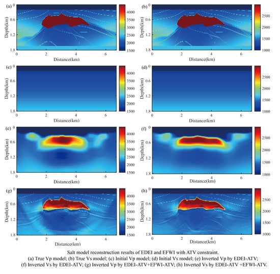
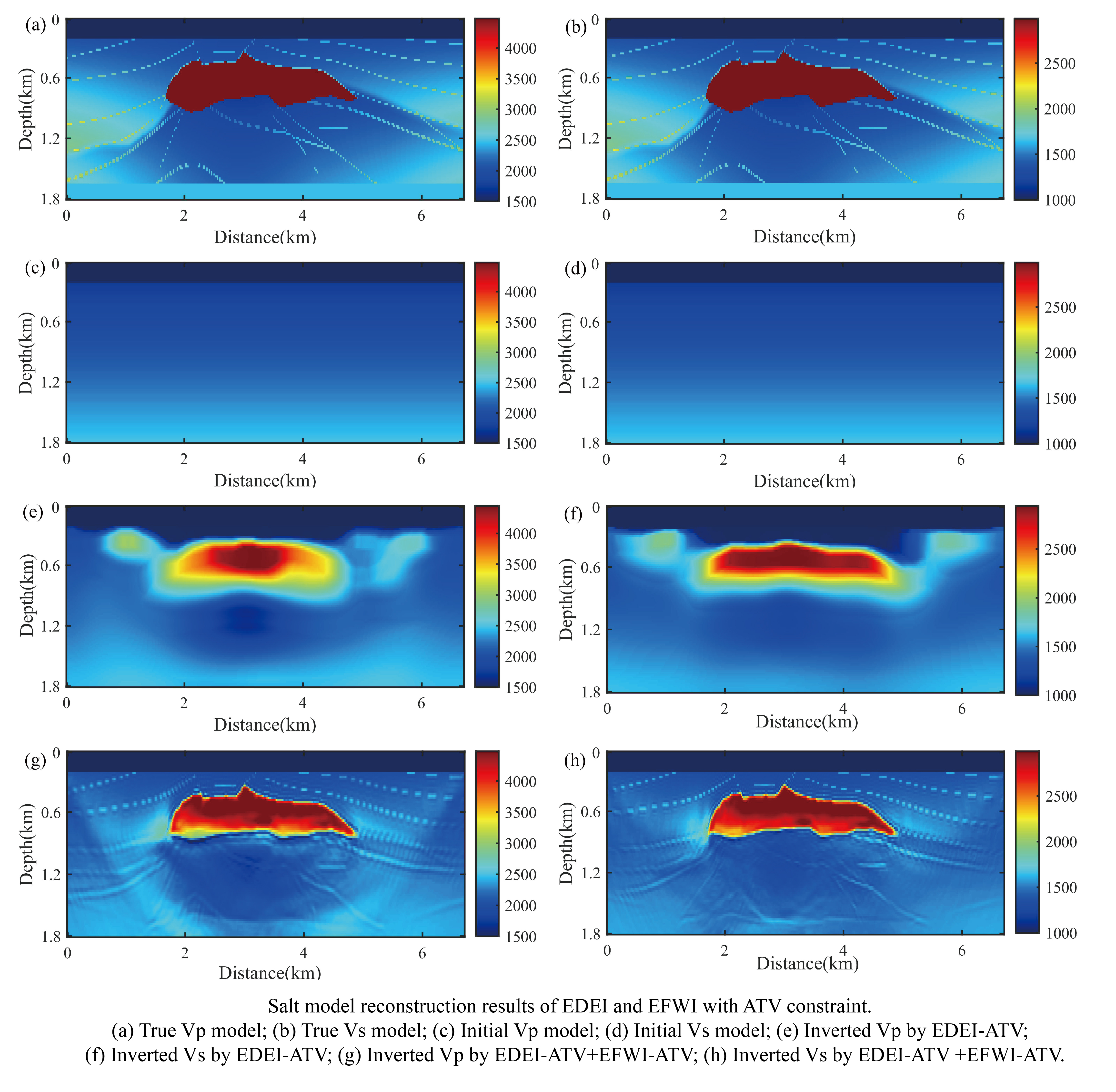
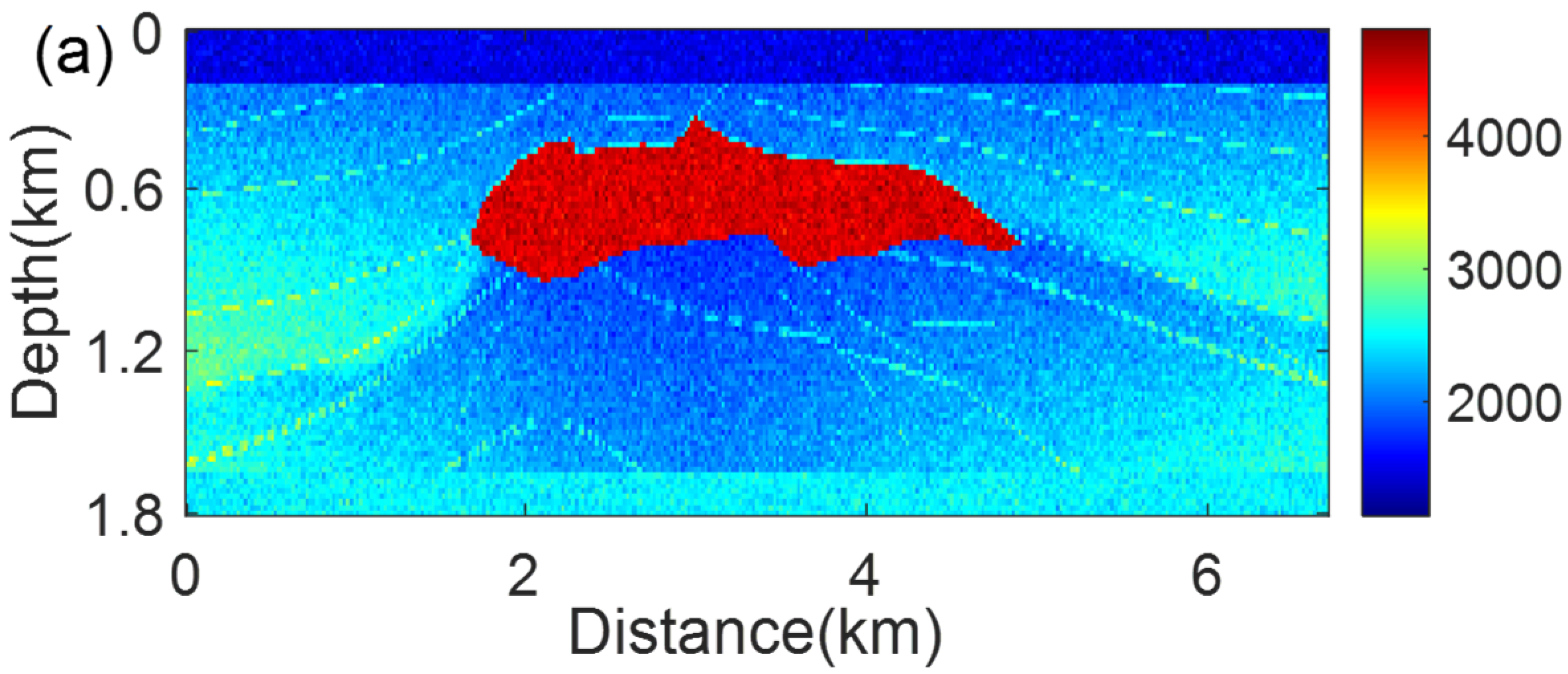
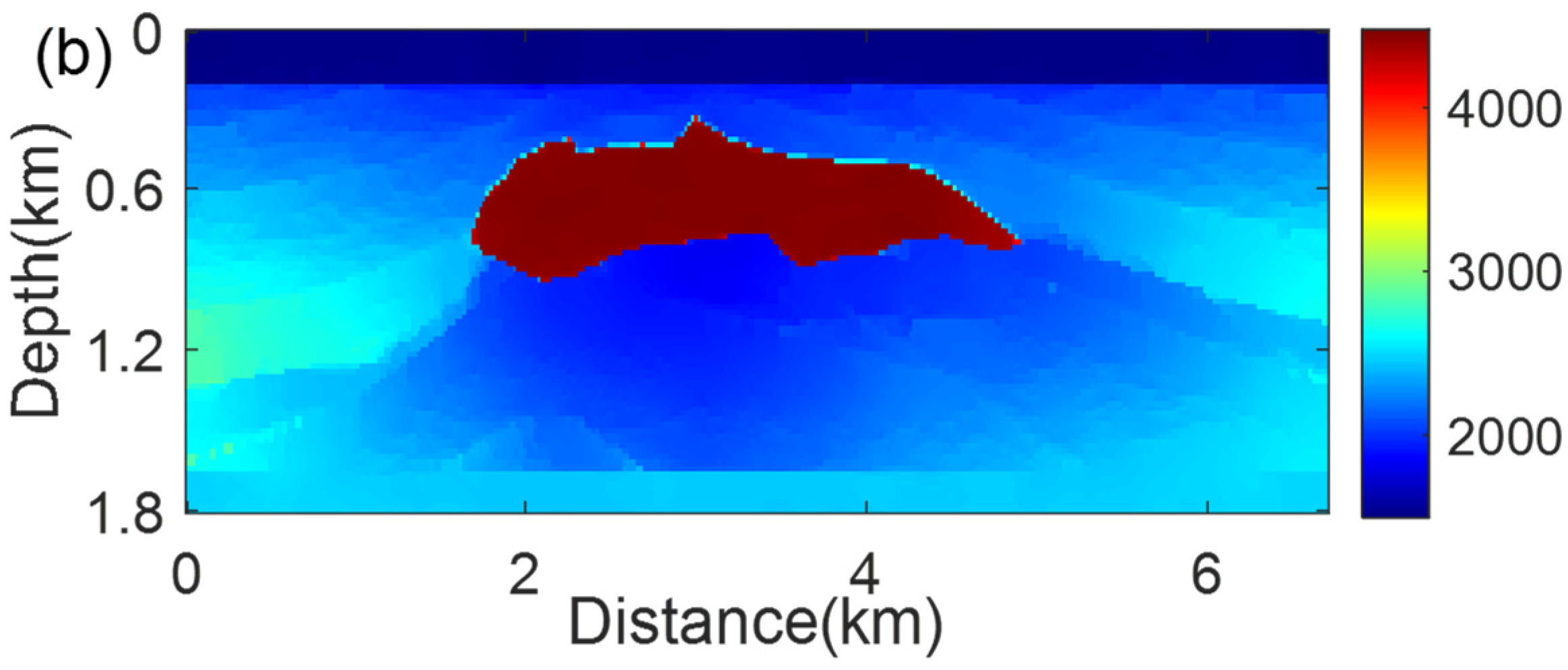
4. Numerical Examples

We test the inversion effects of the proposed method on a modified SEG/EAGE salt dome model. The true Vp and Vs models are shown in Figure 2a,b, respectively. The waveform and frequency spectrum of the source wavelet are shown in Figure 3a,b, respectively. The source wavelet is a Ricker wavelet after high-pass filtering, and the low-frequency information below 3 Hz is cut off. The main frequency of the source wavelet is about 9 Hz. The initial velocity models of Vp and Vs are shown in Figure 4a,b, respectively. There is no prior information of strong scatterers in the initial Vp and Vs models.
Conventional EFWI is performed on the initial Vp and Vs models, and the inversion results of Vp and Vs are shown in Figure 5a,b, respectively. We can find that due to the lack of low-frequency information, the conventional EFWI can only recover part of the top boundary of the strong scatterer, and cannot recover the interior velocity and shape information of the strong scatterer.
Starting with the velocity models shown in Figure 4, the unconstrained EDEI method is carried out. The results of Vp and Vs are shown in Figure 6a,b, respectively. It shows that although the shape of strong scatterers has been restored to a certain extent, the internal velocity of the salt dome still deviates from the true value. In the unconstrained condition, the results in Figure 6a,b are used as the initial model, and the conventional EFWI is performed. The final Vp and Vs inversion results are shown in Figure 6c,d. We can see that the velocity uniformity inside the salt dome is not good, and the lower boundary of the salt dome is not fully described.
Taking the models shown in Figure 4 as the initial model, the EDEI-ATV method is performed, and the obtained Vp and Vs models are shown in Figure 6e,f. We can see that the large-scale Vp and Vs structures of the strong scatterers have been successfully recovered, and the velocity information inside the salt dome is relatively close to the true value. Using Figure 6e,f as initial models, the EFWI-ATV method is performed, and the final Vp and Vs results are shown in Figure 6g,h. It shows that the boundary information and internal velocity of strong scatterers are well retrieved. The inversion effects of the interior velocity, lower boundary and subsalt area of the salt dome are better than that of the unconstrained case.
To further compare the inversion results in Figure 6, we plot some extracted traces, as shown in Figure 7. For the large-scale velocity construction effect, the Vp and Vs inversion results with ATV constraint are closer to the true model. The construction result of Vs model is better than that of Vp model. For the final inversion results, the inversion results with ATV constraint are better than those without constraints, whether in the interior or at the boundary of the salt dome. The inversion effect of Vs is better than that of Vp. The final results still have a good recovery of subsalt structures.
The adjoint sources of conventional EFWI and EDEI are shown in Figure 8. In Figure 8a,b, we can see clear residual reflections because the initial models are linear gradient models without reflection layers. The adjoint sources in Figure 8c,d are very different from those in Figure 8a,b. The frequency band of the residuals is obviously lower and mainly reflects large-scale scattering information. The data fitting results of the inverted velocity models are shown in Figure 9. We can see that after conventional inversion, there are relatively strong residuals in the difference profiles (Figure 9c,h) of the observed data and synthetic data. The difference profiles (Figure 9e,j) corresponding to the ATV constraint inversion results has weaker residuals, which demonstrates that the ATV constraint inversion results are better solutions compared with the conventional inversion results.

5. Discussion and Conclusions

From the numerical examples above, we can see obvious improvements on the elastic strong-scattering media reconstruction of the SEG/EAGE salt model. However, when dealing with field data application, we may face some difficult problems, such as noises, amplitude mismatch, source wavelet error, complex background structures, etc. Real noise such as random noise and ground rolls should be removed before inversion. EDEI and EFWI have the intrinsic ability to suppress a moderate level of random noise, but regular noise such as ground rolls can be a problem and lead to bad results. The data processing techniques and density change will influence the amplitude of the observed data. Considering density inversion is a good way to reduce its effects on amplitude matching. When only considering the global change of data amplitude, the global correlation misfit function is a good choice to ensure a good convergence. The source wavelet is the beginning condition of the forward modeling algorithm, so it is an important factor for the inversion process. A good source wavelet estimation and the source-independent inversion methods are both effective ways to mitigate the effects of source wavelet errors on the inversion results.
In this paper, we propose an EDEI method with anisotropic total variation constraint. The anisotropic total variational constraint is beneficial to make the internal velocity of the structure uniform and the boundary sharp, which can improve the inversion effect of the large-scale velocity structures of the salt dome. The anisotropic total variational constraint problem and the inverse problem can be calculated alternately to achieve good constraint effects. In this paper, the anisotropic total variational constraint is imposed on the inverted Vp and Vs models, respectively. Using the EDEI-ATV inversion results as the initial velocity models, the EFWI-ATV process can obtain better velocity construction of the salt dome. The inversion results show that the depiction of the interior and boundary of the salt dome has been significantly improved.

Author Contributions

Conceptualization, P.Z. and R.-S.W.; methodology, P.Z. and R.-S.W.; software, P.Z; validation, L.H.; formal analysis, P.Z. and L.H.; investigation, P.Z.; resources, P.Z.; data curation, P.Z.; writing—original draft preparation, P.Z.; writing—review and editing, P.Z., R.-S.W. and L.H.; visualization, P.Z., Y.Z.; supervision, P.Z., R.-S.W. and L.H.; project administration, P.Z. and L.H.; funding acquisition, P.Z., R.-S.W. and L.H. All authors have read and agreed to the published version of the manuscript.

Funding

This research was funded by the National Natural Science Foundation of China, grant number 42004106, 42130805 and 42074154, the Natural Science Foundation of Jilin Province, grant number YDZJ202101ZYTS020, the Second Tibetan Plateau Scientific Expedition and Research Program (STEP), grant number 2019QZKK0701-02, the National Key R&D Program of China, grant number 2020YFE0201300, the Lift Project for Young Science and Technology Talents of Jilin Province, grant number QT202116.

Institutional Review Board Statement

Not applicable.

Informed Consent Statement

Not applicable.

Data Availability Statement

Data supporting reported results are available by contacting the corresponding author.

Conflicts of Interest

The authors declare no conflict of interest.

References

  1. Tarantola, A. Inversion of seismic reflection data in the acoustic approximation. Geophysics 1984, 49, 1259–1266. [Google Scholar] [CrossRef]
  2. Virieux, J.; Operto, S. An overview of full-waveform inversion in exploration geophysics. Geophysics 2009, 74, WCC127–WCC152. [Google Scholar] [CrossRef]
  3. Rivera, C.; Trinh, P.; Bergounioux, E.; Duquet, B. Elastic multiparameter FWI in sharp contrast medium. In Proceedings of the 89th SEG Annual Meeting, San Antonio, TX, USA, 15–20 September 2019. [Google Scholar]
  4. Shin, C.; Cha, Y.H. Waveform inversion in the Laplace domain. Geophys. J. Int. 2008, 173, 922–931. [Google Scholar] [CrossRef] [Green Version]
  5. Shin, C.; Cha, Y.H. Waveform inversion in the Laplace-Fourier domain. Geophys. J. Int. 2009, 177, 1067–1079. [Google Scholar] [CrossRef]
  6. Lewis, W.; Starr, B.; Vigh, D. A level set approach to salt geometry inversion in full-waveform inversion. In Proceedings of the 82nd SEG Annual Meeting, Las Vegas, NV, USA, 4–9 November 2012. [Google Scholar]
  7. Chen, S.; Chen, G. Full waveform inversion based on time-integral-dam** wavefield. J. Appl. Geophys. 2019, 163, 84–95. [Google Scholar] [CrossRef]
  8. Yang, F.; Ma, J. Deep-learning inversion: A next-generation seismic velocity model building method. Geophysics 2019, 84, R583–R599. [Google Scholar] [CrossRef] [Green Version]
  9. Anagaw, A.; Sacchi, M. Edge-preserving smoothing for simultaneous-source full-waveform inversion model updates in high-contrast velocity models. Geophysics 2018, 83, A33–A37. [Google Scholar] [CrossRef]
  10. Chai, X.; Tang, G.; Peng, R.; Liu, S. The linearized Bregman method for frugal full-waveform inversion with compressive sensing and sparsity-promoting. Pure Appl. Geophys. 2018, 175, 1085–1101. [Google Scholar] [CrossRef]
  11. Askan, A.; Akcelik, V.; Bielak, J.; Ghattas, O. Full waveform inversion for seismic velocity and anelastic losses in heterogeneous structures. Bull. Seismol. Soc. Amer. 2007, 97, 1990–2008. [Google Scholar] [CrossRef] [Green Version]
  12. Lin, Y.; Huang, L. Acoustic- and elastic-waveform inversion using a modified total-variation regularization scheme. Geophys. J. Int. 2015, 200, 489–502. [Google Scholar] [CrossRef] [Green Version]
  13. Zhang, P.; Han, L.; Gong, X.; Sun, H.; Mao, B. Multi-source elastic full waveform inversion based on the anisotropic total variation constraint. Chin. J. Geophys. -Chin. Ed. 2018, 61, 716–732. [Google Scholar]
  14. Qu, S.; Verschuur, E.; Chen, Y. Full-waveform inversion and joint migration inversion with an automatic directional total variation constraint. Geophysics 2019, 84, R175–R183. [Google Scholar] [CrossRef]
  15. Aghamiry, H.; Gholami, A.; Operto, S. Multiparameter wavefield reconstruction inversion for wavespeed and attenuation with bound constraints and total variation regularization. Geophysics 2020, 85, R381–R396. [Google Scholar]
  16. Feng, D.; Wang, X.; Wang, X. New dynamic stochastic source encoding combined with a minmax-concave total variation regularization strategy for full waveform inversion. IEEE Trans. Geosci. Remote Sens. 2020, 58, 7753–7771. [Google Scholar] [CrossRef]
  17. Zhang, T.; Sun, J.; Innanen, K.A.; Trad, D.O. A recurrent neural network for 1 anisotropic viscoelastic full waveform inversion with high-order total variation regularization. In Proceedings of the First International Meeting for Applied Geoscience & Energy, Denver, CO, USA, 27 August–1 September 2021. [Google Scholar]
  18. Esser, E.; Herrmann, F.J.; Guasch, L.; Warner, M. Constraint waveform inversion in salt-affected datasets. In Proceedings of the 85th SEG Annual Meeting, New Orleans, LA, USA, 18–23 October 2015. [Google Scholar]
  19. Esser, E.; Guasch, L.; Herrmann, F.J.; Warner, M. Constrained waveform inversion for automatic salt flooding. Lead. Edge 2016, 35, 235–239. [Google Scholar] [CrossRef]
  20. Qiu, L.; Chemingui, N.; Zou, Z.; Valenciano, A. Full waveform inversion with steerable variation regularization. In Proceedings of the 86th SEG Annual Meeting, Dallas, TX, USA, 16–21 October 2016. [Google Scholar]
  21. Peters, B.; Herrmann, F.J. Constraints versus penalties for edge-preserving full-waveform inversion. Lead. Edge 2017, 36, 94–100. [Google Scholar] [CrossRef]
  22. Yong, P.; Liao, W.; Huang, J.; Li, Z. Total variation regularization for seismic waveform inversion using an adaptive primal dual hybrid gradient method. Inverse Probl. 2018, 34, 045006. [Google Scholar] [CrossRef]
  23. Kalita, M.; Kazei, V.; Choi, Y.; Alkhalifah, T. Regularized full-waveform inversion with automated salt flooding. Geophysics 2019, 84, R569–R582. [Google Scholar] [CrossRef] [Green Version]
  24. Wu, R.S.; Luo, J.; Wu, B. Seismic envelope inversion and modulation signal model. Geophysics 2014, 79, WA13–WA24. [Google Scholar] [CrossRef]
  25. Luo, J.R.; Wu, R.S. Seismic envelope inversion: Reduction of local minima and noise resistance. Geophys. Prospect. 2015, 63, 597–614. [Google Scholar] [CrossRef]
  26. Bozdag, E.; Trampert, J.; Tromp, J. Misfit functions for full waveform inversion based on instantaneous phase and envelope measurements. Geophys. J. Int. 2011, 185, 845–870. [Google Scholar] [CrossRef]
  27. Zhang, P.; Wu, R.S.; Han, L. Seismic envelope inversion based on hybrid scale separation for data with strong noises. Pure Appl. Geophys. 2019, 176, 165–188. [Google Scholar] [CrossRef]
  28. Wu, R.S.; Chen, G. New Fréchet derivative for envelope data and multi-scale envelope inversion. In Proceedings of the 79th EAGE Annual Meeting, Paris, France, 12–15 June 2017. [Google Scholar]
  29. Wu, R.S.; Chen, G. Multi-Scale Seismic Envelope Inversion Using a Direct Envelope Fréchet Derivative for Strong-Nonlinear Full Waveform Inversion. 2018. Available online: https://arxiv.org/abs/1808.05275 (accessed on 20 November 2022).
  30. Wu, R.S. Towards a Theoretical Background for Strong-Scattering Inversion—Direct Envelope Inversion and Gel’fand-Levitan-Marchenko Theory. Commun. Comput. Phys. 2020, 28, 41–73. [Google Scholar]
  31. Chen, G.; Wu, R.S.; Chen, S. Reflection multi-scale envelope inversion. Geophys. Prospect. 2018, 66, 1258–1271. [Google Scholar] [CrossRef]
  32. Chen, G.; Wu, R.S.; Wang, Y.; Chen, S. Multi-scale signed envelope inversion. J. Appl. Geophys. 2018, 153, 113–126. [Google Scholar] [CrossRef]
  33. Wang, Y.; Wu, R.S.; Chen, G.; Peng, Z. Seismic modulation model and envelope inversion with smoothed apparent polarity. J. Geophys. Eng. 2018, 15, 2278–2286. [Google Scholar] [CrossRef] [Green Version]
  34. Chen, G.; Yang, W.; Chen, S.; Liu, Y.; Gu, Z. Application of envelope in salt structure velocity building: From objective function construction to the full-band seismic data reconstruction. IEEE Trans. Geosci. Remote Sens. 2020, 58, 6594–6608. [Google Scholar] [CrossRef]
  35. Zhang, P.; Wu, R.S.; Han, L. Source-independent seismic envelope inversion based on the direct envelope Fréchet derivative. Geophysics 2018, 83, R581–R595. [Google Scholar] [CrossRef]
  36. Chen, G.; Wu, R.S.; Chen, S. Multiscale direct envelope inversion: Algorithm and methodology for application to the salt structure inversion. Earth Space Sci. 2019, 6, 174–190. [Google Scholar] [CrossRef] [Green Version]
  37. Hu, Y.; Wu, R.S.; Han, L.; Zhang, P. Joint multiscale direct envelope inversion of phase and amplitude in the time-frequency domain. IEEE Trans. Geosci. Remote Sens. 2019, 57, 5108–5120. [Google Scholar] [CrossRef]
  38. Luo, J.; Wu, R.S.; Chen, G. Angle domain direct envelope inversion method for strong-scattering velocity and density estimation. IEEE Geosci. Remote Sens. Lett. 2020, 17, 1508–1512. [Google Scholar] [CrossRef]
  39. Zhang, P.; Han, L.; Zhang, F.; Feng, Q.; Chen, X. Wavefield decomposition-based direct envelope inversion and structure-guided perturbation decomposition for salt building. Minerals 2021, 11, 919. [Google Scholar] [CrossRef]
  40. Zhang, P.; Wu, R.S.; Han, L.; Hu, Y. Elastic direct envelope inversion based on wave mode decomposition for multi-parameter reconstruction of strong-scattering media. Pet. Sci. 2022, 19, 2046–2063. [Google Scholar] [CrossRef]
  41. Luo, J.; Wu, R.S.; Hu, Y.; Chen, G. Strong scattering elastic full waveform inversion with the envelope Fréchet derivative. IEEE Geosci. Remote Sens. Lett. 2022, 19, 8008805. [Google Scholar] [CrossRef]
  42. Chen, G.; Yang, W.; Liu, Y.; Wang, H.; Huang, X. Salt structure elastic full waveform inversion based on the multiscale signed envelope. IEEE Trans. Geosci. Remote Sens. 2022, 60, 1–12. [Google Scholar] [CrossRef]
  43. Zhang, P.; **ng, Z.; Hu, Y. Velocity construction using active and passive multi-component seismic data based on elastic full waveform inversion. Chin. J. Geophys. -Chin. Ed. 2019, 62, 3974–3987. [Google Scholar]
  44. Beck, A.; Teboulle, M. Fast gradient-based algorithms for constrained total variation image denoising and deblurring problems. IEEE Trans. Image Process. 2009, 18, 2419–2434. [Google Scholar] [CrossRef] [Green Version]
Figure 1. ATV constraint denoising test. (a) Salt velocity model with random noise; (b) ATV constraint denoising result.
Remotesensing 15 00746 g001aRemotesensing 15 00746 g001b
Figure 2. The modified SEG/EAGE salt dome model for elastic media. (a) True Vp model; (b) True Vs model.
Remotesensing 15 00746 g002
Figure 3. Source wavelet and its spectrum. (a) Waveform of source wavelet; (b) Spectrum of source wavelet.
Remotesensing 15 00746 g003
Figure 4. Initial velocity model. (a) Initial Vp model; (b) Initial Vs model.
Remotesensing 15 00746 g004
Figure 5. Inversion results of conventional EFWI. (a) Inverted Vp result; (b) Inverted Vs result.
Remotesensing 15 00746 g005
Figure 6. Inversion results with and without ATV constraint. (a) Inverted Vp by EDEI; (b) Inverted Vs by EDEI; (c) Inverted Vp by EDEI + EFWI; (d) Inverted Vs by EDEI + EFWI; (e) Inverted Vp by EDEI-ATV; (f) Inverted Vs by EDEI-ATV; (g) Inverted Vp by EDEI-ATV + EFWI-ATV; (h) Inverted Vs by EDEI-ATV + EFWI-ATV.
Remotesensing 15 00746 g006
Figure 7. Extracted traces comparison of inversion results. (a) Extracted traces comparison of inverted Vp by EDEI and EDEI-ATV; (b) Extracted traces comparison of inverted Vs by EDEI and EDEI-ATV; (c) Extracted traces comparison of inverted Vp by EDEI+EFWI and EDEI-ATV + EFWI-ATV; (d) Extracted traces comparison of inverted Vs by EDEI + EFWI and EDEI-ATV + EFWI-ATV.
Remotesensing 15 00746 g007aRemotesensing 15 00746 g007b
Figure 8. Adjoint sources comparison. (a) Z-component of the adjoint source of EFWI; (b) X-component of the adjoint source of EFWI; (c) Z-component of the adjoint source of EDEI; (d) X-component of the adjoint source of EDEI.
Remotesensing 15 00746 g008
Figure 9. Data fitting results. (a) Z-component observed data; (b) Z-component synthetic data on Figure 6c,d; (c) Difference profile of Figure 9a,b; (d) Z-component synthetic data on Figure 6g,h; (e) Difference profile of Figure 9a,d; (f) X-component observed data; (g) X-component synthetic data on Figure 6c,d; (h) Difference profile of Figure 9f,g; (i) X-component synthetic data on Figure 6g,h; (j) Difference profile of Figure 9f,i.
Remotesensing 15 00746 g009aRemotesensing 15 00746 g009b
Disclaimer/Publisher’s Note: The statements, opinions and data contained in all publications are solely those of the individual author(s) and contributor(s) and not of MDPI and/or the editor(s). MDPI and/or the editor(s) disclaim responsibility for any injury to people or property resulting from any ideas, methods, instructions or products referred to in the content.

