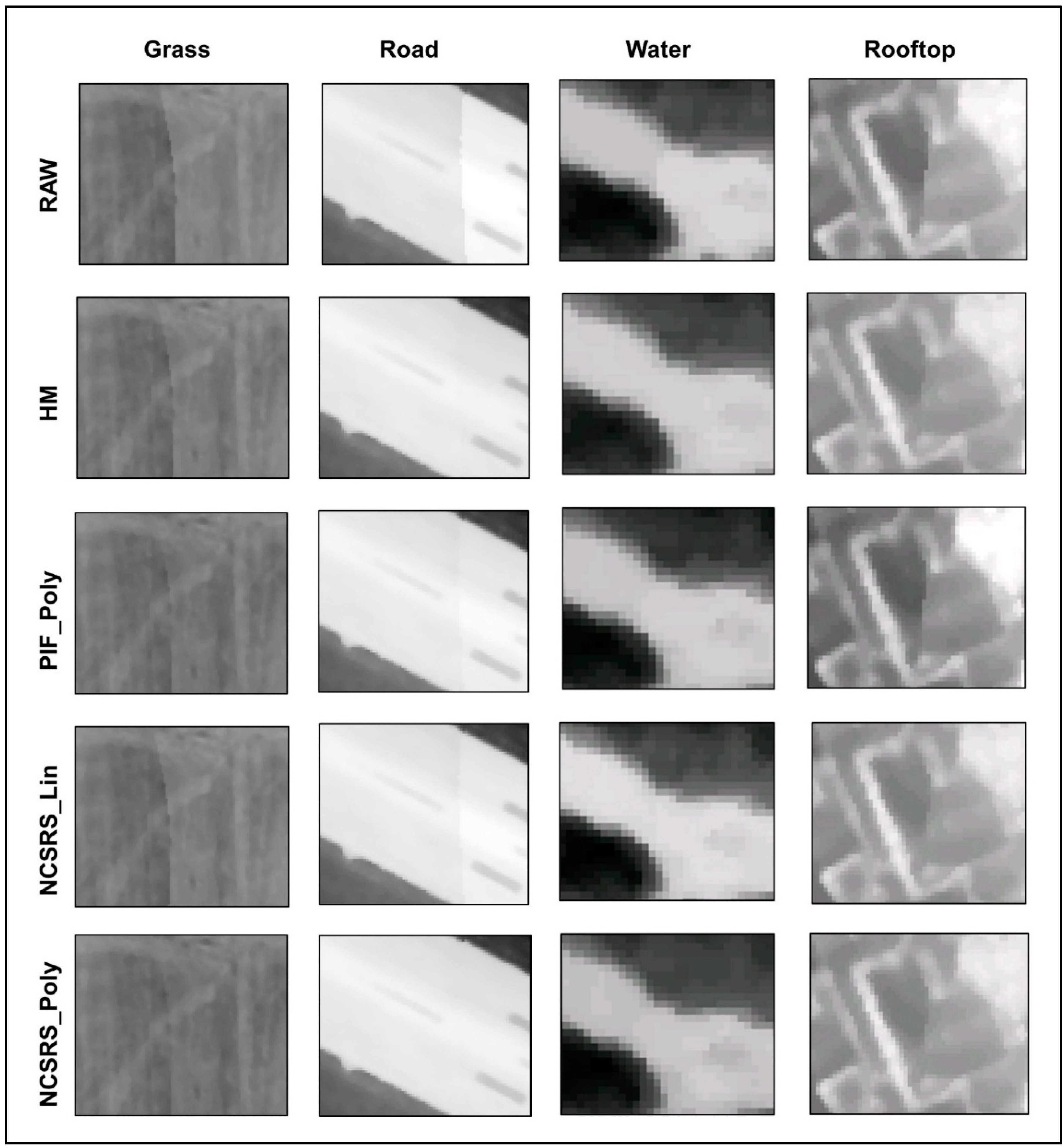
3.1. Visual Assessments
Visual assessment is a straightforward way to judge the performance of the evaluated methods. In so doing, the master and the slave flight lines were joined and features along the mosaic line were assessed. If the visual differences between the master and the normalized slave images are smaller than that of the master and the raw slave images, the normalized image can be considered as radiometrically fitted to the reference image.
A visual assessment of grass, road, water and rooftop samples (illustrated in
Figure 5) shows that each tested method visually improves the radiometric agreement between the master and the slave images compared to the raw image. However, the degree of normalization varies depending on the method used and the land cover type assessed. Specifically:
- ▪
HM appears to perform very well for road and water, but performs only moderately well for grass and rooftop.
- ▪
PIF_Poly performs well for road and water and moderately well for grass, but it does not perform well for rooftop.
- ▪
NCSRS_Lin performs very well for water and moderately well for road, grass and rooftop.
- ▪
NCSRS_Poly performs very well for road and water and well for grass and rooftop. Though subjective, we further suggest that grass and rooftop visually appear best modeled by this method.
Figure 5.
Visual examples of four different relative radiometric normalization methods applied along the mosaic join line of four different land cover types (grass, road, water and rooftop). PIF_Poly—pseudo-invariant feature-based polynomial regression; NCSRS_Lin-no-change stratified random sample-based linear regression.
In general, the radiometric error of geographically simple features, like road and water, are visually reduced by all methods; this, in part, can be explained by their high thermal inertia, which results in low within-class variability (regardless of their acquisition time within either flight line).
We also note that while the river water class is a part of a dynamic system, its nighttime temperature fluctuates very little as its source is regulated by high mountain snow melt. However, complex features, like grass and rooftops, are not well modeled by most of the evaluated methods. This, in part, can be explained by their complex and variable nature. That is: (i) Different types of grass will exhibit different nighttime evapotranspiration rates; and (ii) the temperature of different roof sections (even for the same building structure) can be differentially heated at different times during the night, as they respond to varying local microclimatic differences in temperature and humidity—two attributes typically assessed by modern in-home thermostats. At a broader community scale, roof tops can further be considered a highly variable land cover feature, as they are composed of numerous materials, many of which have different emissivity characteristics that need to be corrected for (after radiometric normalization) in order to convert their relative temperature values (defined by the sensor) to true kinetic temperatures [
2,
3]. As a consequence, a small constant difference in (relative) ambient temperature may result in several degrees of difference in roofs composed of different materials, which are not corrected for emissivity.
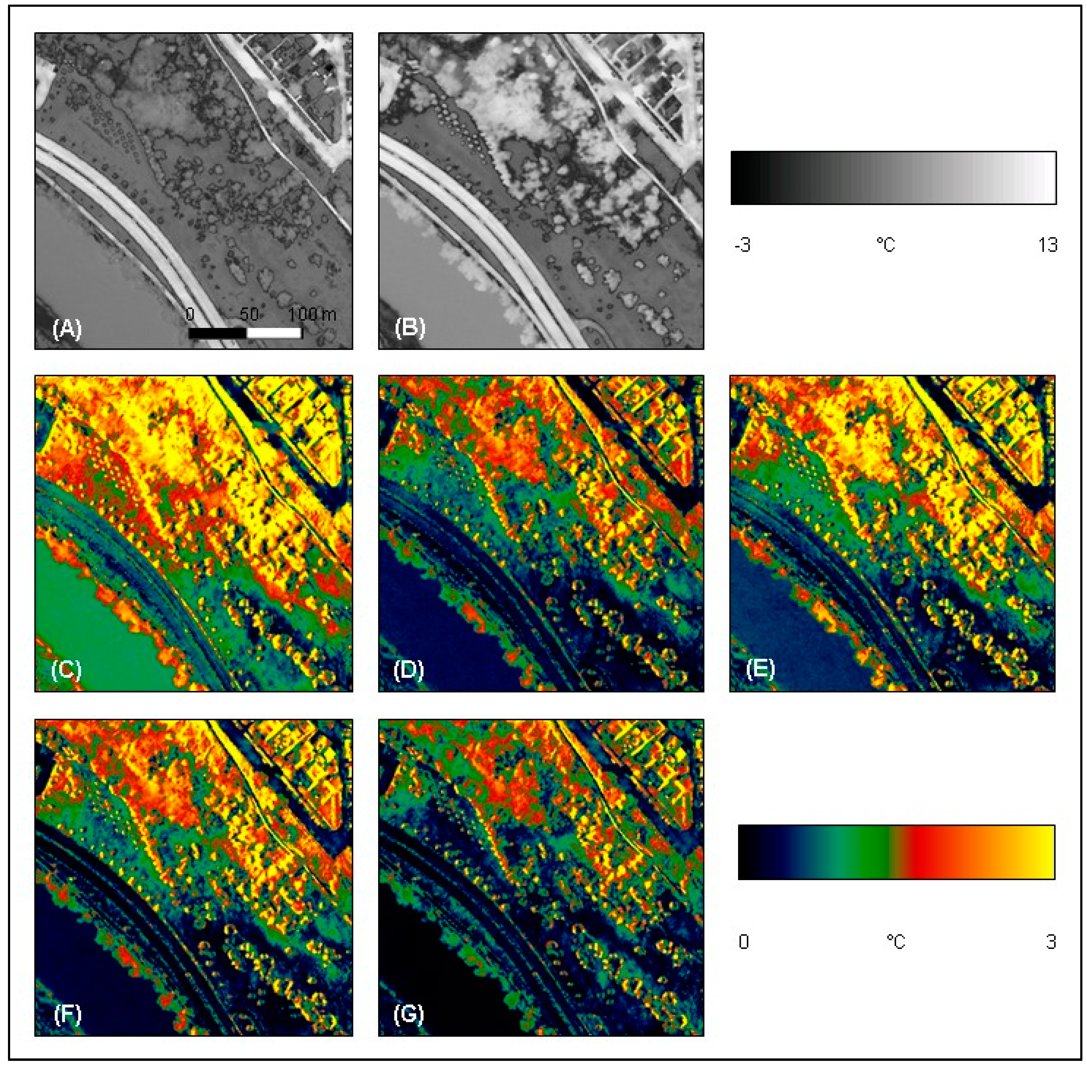
Figure 6 provides another visual example of how the four evaluated relative radiometric normalization techniques reduce the thermal variability between the master and slave image(s) for four different land cover types.
Figure 6A (the master) and 6B (the slave) represent corresponding grey-scale TABI-1800 image samples of a small area located within the flight line overlap that is predominantly composed of vegetation, roads, a (water-body) river and roofs. In both of these grey-scale sub-images, grass (smooth lower right) and roofs (top right corner) appear cool (mid-dark grey), the river (lower left diagonal feature) and trees (textured blobs) are moderately warm (light grey), while roads and paths are the hottest (white). In
Figure 6C, the strongest temperature difference between the master and the uncorrected (raw) slave image appears yellow (+3 °C) for trees and rooftops. However after radiometric normalization, these differences and those of other features tend to visually decrease (
Figure 6D–G). For example, water and road appear well modeled by most of the methods, displaying a minimum difference (
i.e., black or blue ≈ 0–1 °C) between the master and the normalized slave images. Overall, rooftops and trees display the highest differences (yellow ≈ +3 °C), which perpetuates over different spatial extents in all slave images. Upon more detailed visual inspection, these yellow coloured rooftops and trees appears to be due to geometric shift-differences, especially noticeable as yellow regions along the edge of buildings (see the top right
Figure 6D–G) and on tree-tops and along paths (within the same figures). However, based on a visual assessment of the pseudo-coloured temperature differences for all of the RRN samples, NCSRS_Poly visually appears to perform the best for all four land cover types (as it exhibits the most black and blue colors, thus representing the smallest temperature differences), closely followed by HM and NCSRS_Lin.
Figure 6.
A visual example of how relative radiometric normalization techniques decrease the radiometric variability between flight lines. (A) A sample area from the master image. (B) The same area from the slave image. Pseudo-colored absolute image difference (C) between the master and the uncorrected slave image and between the master and the normalized salve images resulting from (D) HM, (E) PIF_Poly, (F) NCSRS_Lin and (G) NCSRS_Poly.
3.2. Statistical Analysis
As noted in
Section 2.2.4, the root mean square error (
RMSE) was used to define the statistical agreement between the normalized slave images and the master image. This required collecting 2000 stratified random sample points within the overlap that represent four different land cover types over a wide range of temperatures. These include: (i) grass; (ii) road; (iii) water; and (iv) rooftop.
Table 1 summarizes the
RMSEs calculated for these cover types.
Table 1.
The overall RMSE of four different land cover types, for each of the four different relative radiometric normalization methods evaluated in this study. Bold values represent the lowest RMSE of each class and overall RMSE calculated for each image.
Table 1.
The overall RMSE of four different land cover types, for each of the four different relative radiometric normalization methods evaluated in this study. Bold values represent the lowest RMSE of each class and overall RMSE calculated for each image.
| Land Cover Type | RMSE (°C) |
|---|
| Slave | HM | PIF_Poly | NCSRS_Lin | NCSRS_Poly |
|---|
| Grass | 0.420 | 0.236 | 0.227 | 0.193 | 0.163 |
| Road | 0.201 | 0.097 | 0.128 | 0.122 | 0.123 |
| Rooftop | 0.586 | 0.436 | 0.452 | 0.371 | 0.322 |
| Water | 0.216 | 0.106 | 0.108 | 0.130 | 0.113 |
| Overall * | 0.356 | 0.194 | 0.210 | 0.173 | 0.159 |
In general, all methods show a reduced radiometric variation between the master and the slave images. From
Table 1, we see that complex features, like rooftops and grass, have higher
RMSE values in the uncorrected slave image than other features. This is understandable, as different roofing materials are used in Calgary, including asphalt shingles, clay tiles, cedar, tar and gravel, wood, concrete, fibreglass, vinyl shingles,
etc. each of which have different thermal capacities, conductivity and emissivity. As a result, we found it challenging to radiometrically normalize rooftops with each of the methods. Similarly, the grass class also has a higher
RMSE in the uncorrected slave image, potentially due to: (i) the various species compositions, each with varying allometric and morphometric characteristics; and (ii) the varying amount of moisture in the background soil [
28]. The other two features (road and water) are relatively simple and exhibit relatively lower
RMSE values in the slave image. They are also reasonably well modeled by all methods, resulting in decreased
RMSE values (~50%). However, the complex feature classes (rooftop and grass) are best modeled only by the NCSRS-based methods, with the NCSRS-based polynomial technique providing the lowest overall
RMSE values (0.322 and 0.163 respectively).
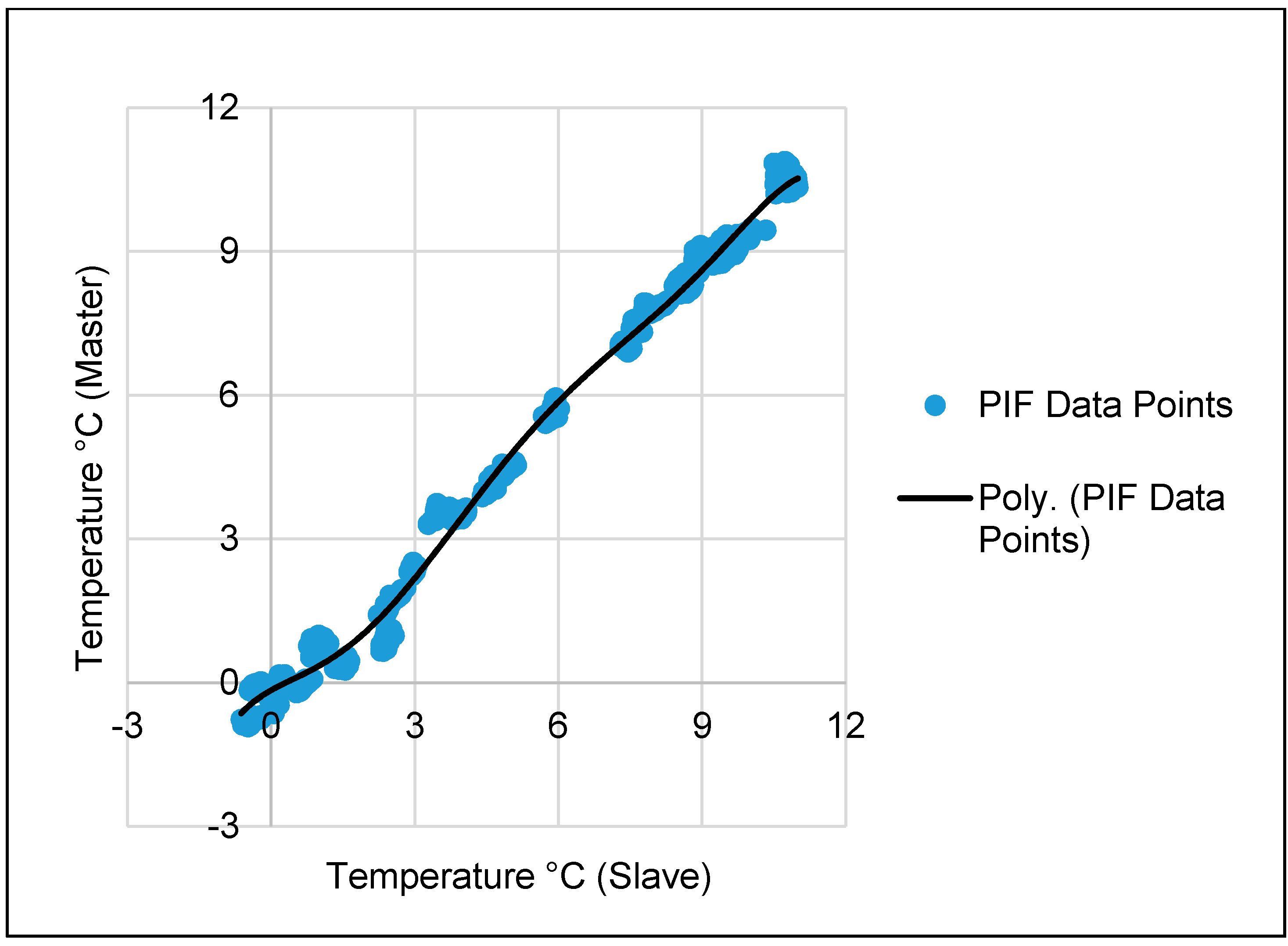
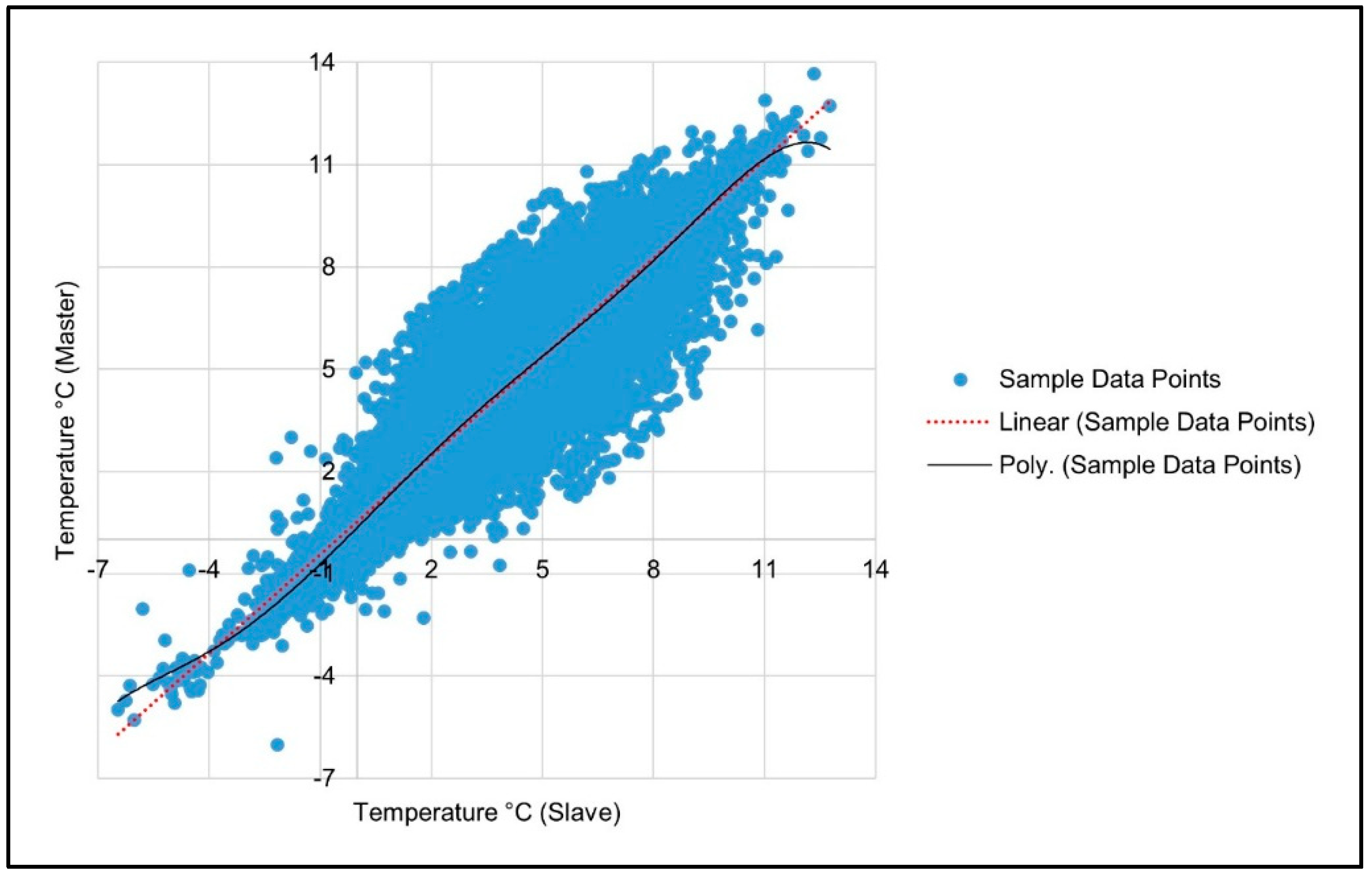
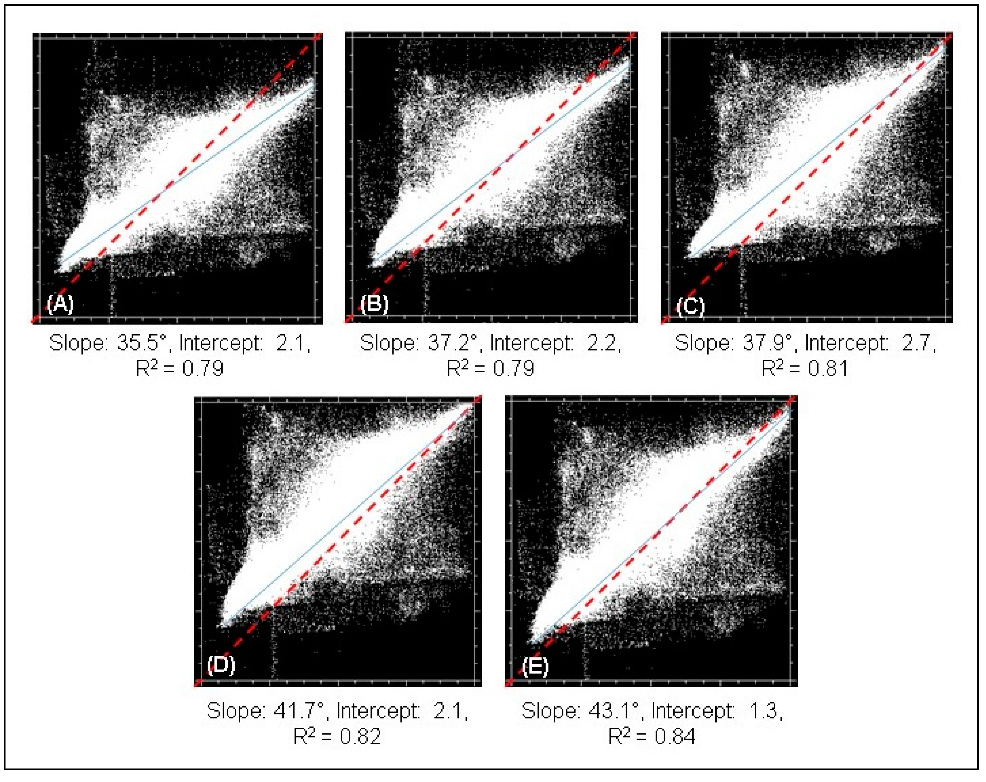
Figure 7 illustrates the scatterplots and resulting trend-lines between the master and the slave images before (
Figure 7A) and after (
Figure 7B–E) normalization. The blue lines represent the linear trend lines, while the red dashed lines illustrate the expected trend of each dataset at perfect radiometric agreement. Scatterplots can be used to describe various correlations between different variables. A high positive linear correlation exists between two datasets when the data cloud follows a 45° diagonal line (
i.e., the red dotted line in
Figure 7A–E). This indicates that the datasets are not only highly correlated, but also that their DN values are very close to each other.
In a perfect scenario, if two datasets represent the same features, their slope in the scatterplot should be 45° and their intercept should be at zero. In the scatterplot of the raw images (
Figure 7A), the slope is shown to be 35.5° and the intercept is shown as 2.1. However, each of the normalized scatterplots (
Figure 7B–E) improves the slope between the master and the slave, and most of the methods improve both the intercept and the slope. Of those methods tested, the scatterplot results (
Figure 7A–E) show that the NCSRS_Poly trend line (
Figure 7E) is visually and statistically the closest to the red line with a slope of 43.1°, an intercept of 1.3 and an R
2 of 0.84. Thus, it represents the best performing normalization method, followed by NCSRS_Lin (
Figure 7D). Conversely, while the HM method improves the slope between the master and the slave (indicating that the radiometric agreement is supposed to improve), the intercept is slightly increased, and in the case of PIF_Poly, the intercept is further increased (meaning that the radiometric agreement is supposed to be decreased).
Figure 7.
(A) A comparison of the scatterplot between the original master and the slave images and after applying four normalization methods: (B) HM; (C) PIF_Poly; (D) NCSRS_Lin; and (E) NCSRS_Poly. The thin blue lines describe the data trend line, while the red dashed lines show the expected trend(s) at perfect radiometric agreement.
3.2.1. A Comparison of Automatic vs Manual Methods
When automatic methods (HM, NCSRS_Lin and NCSRS_Poly) are compared against the manual method (PIF_Poly), the
Table 1 results demonstrate that automated methods are able to more efficiently process large volumes of data, while maintaining a higher level of accuracy (
i.e., a lower
RMSE).
Figure 5 and
Table 1 further show that although the (PIF_Poly) method performed moderately well for grass, road and water, it failed to improve the radiometric agreement for rooftops. Additionally, the required manual collection of samples is time consuming, subject to human error and not easily operationalized for large datasets.
3.2.2. An Assessment of Computation Time
When analyzing large area, H-res TIR imagery, especially within an operational setting, computation time is an important criterion to consider. In order to meaningfully assess the computation times for each of the evaluated radiometric normalization methods, we applied each method over the same datasets and used the same workstation for subsequent analysis. All algorithms were written (in house) in the Interactive Data Language (IDL 8.0) and optimized for performance.
Processing results (
Table 2) show that the NCSRS-based linear regression method required the least amount of time to execute (1.4 min). The second fastest method was histogram matching, which required 2.14 min; while NCSRS_Poly and PIF_Poly each took 4.7 min to compute. However we rate NCSRS_Poly as the third fastest, as its training samples were automatically selected. Conversely, PIF_Poly required the manual collection of training samples, which, in this case, took about 30 min to manually define (from within the overlap between the two flight lines). Furthermore, as the number of flight lines increases, this method becomes increasingly complicated, as additional samples will need to be manually collected from each overlap section. For example, if we were to use this method to process the full City of Calgary with its 43 TABI-1800 fight lines (~600 GB), we estimate 22 h of additional labour, just for manual sample collection (
i.e., 42 overlaps × 30 min each). Thus, we rate PIF_Poly as the slowest method to implement and do not recommend it for large area operational analysis.
Table 2.
Computation time of four different relative radiometric normalization (RRN) methods evaluated in this study.
Table 2.
Computation time of four different relative radiometric normalization (RRN) methods evaluated in this study.
| RRN Method | Computing Time (min) |
|---|
| Histogram Matching | 2.14 |
| PIF_Poly | 4.7 * |
| NCSRS_Lin | 1.4 |
| NCSRS_Poly | 4.7 |
3.2.3. A Comparison of Linear vs Polynomial Methods
In the Introduction, we hypothesized that nonlinear (i.e., polynomial) RRN techniques are better suited to model the temperature variability of complex urban features in H-res TIR imagery than corresponding linear techniques. In this section, we test this hypothesis by comparing only the NCSRS-based linear and polynomial RRN techniques, as they both use the same automatically generated samples in their corresponding regression equations
From a visual assessment of the cover classes in
Figure 5 and
Figure 6 and the scatterplot agreement in
Figure 7, we conclude that NCSRS_Poly visually performs better than NCSRS_Lin. Furthermore,
Table 1 shows the lowest overall
RMSE resulting from NCSRS_Poly. That is, when compared to the original slave test samples (
Table 1), NCSRS_Poly decreases overall
RMSE by 56%, which is 5% less than NCSRS_Lin (51%). However, if we only look at the results for the most complex class (rooftop), NCSRS_Poly decreases the
RMSE by 46%,
vs 36% for NCSRS_Lin.
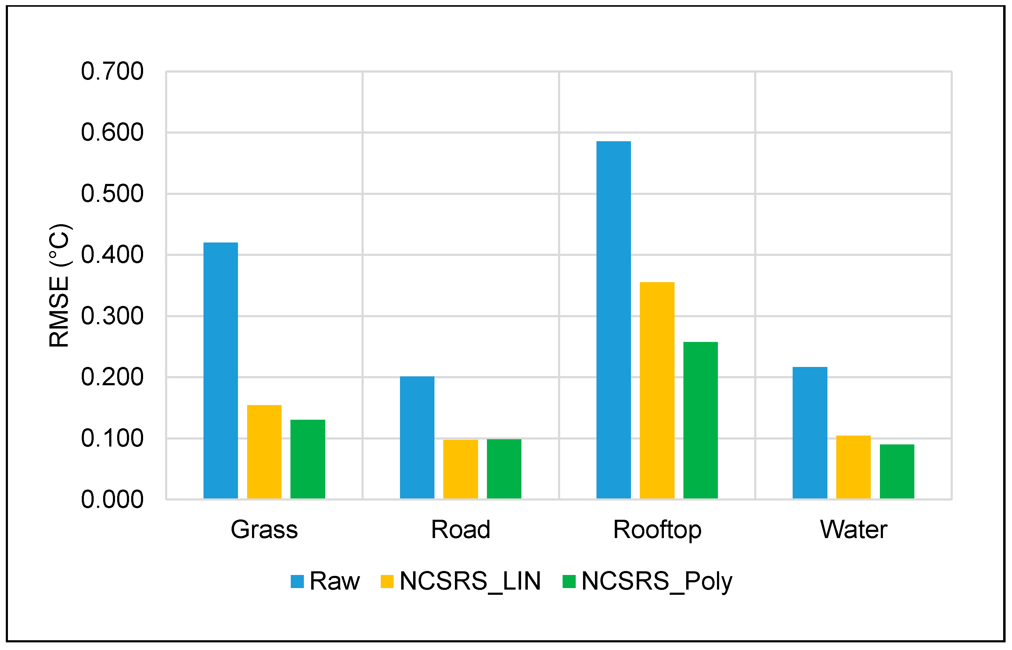
From
Figure 8, we see that results from the polynomial function (in green) display notable improvement over the raw data (blue) or the linear method (yellow) for the two complex land cover classes—grass and rooftop (each of which are characterized by greater internal variability). For more simple landscape features, like water and road, both methods perform very closely, with NCSRS_Poly only slightly better for water.
Figure 8.
A comparison of linear (LIN) and polynomial (Poly) regression-based radiometric normalization using the same no-change stratified random samples (NCSRS).
Figure 8.
A comparison of linear (LIN) and polynomial (Poly) regression-based radiometric normalization using the same no-change stratified random samples (NCSRS).
Based on this combination of results, it is clear that the polynomial technique (NCSRS_Poly) provides improved radiometric agreement over the linear technique, though we note that NCSRS_LIN is three-times faster to implement (see
Table 2). Scaled for 43 flight lines, this represents a processing time of 58.8 min
vs 197.4 min. While a faster implementation time is best, we consider NCSRS_Poly as the most operationally capable, based on the strength of its visual and statistical results, even with its (currently) slower implementation time. If necessary, increased processing speed can be gained from faster hardware.

 ,
, 


