5.1. The Relationship between Observed Ta and Ts from MODIS Terra and Aqua
The influence of the time-of-observation on estimation of Ta has been studied and discussed in several previous studies that resulted different conclusions. For example, Benali
et al. [
4] stated that the use of both Aqua Ts-day and Ts-night could improve the estimation of Tmax and Tmin, respectively, due to the fact that the MODIS Aqua overpass time is closer to the time of both Tmax and Tmin than Terra’s. In contrast, Zhu
et al. [
21] showed that both Terra Ts-day and Ts-night were better than Aqua Ts-day and Ts-night for Ta estimations in **angride River basin of China. In another study, Mostovoy
et al. [
9] found that the difference between satellite overpass (Terra and Aqua) had little impact on the estimation accuracy of Ta.
The comparison between MODIS Ts data and Ta observations shows that Ts-day from both Terra and Aqua, with the mean relative bias above zero, tended to overestimate Tmax (
Table 1). The Ts value of daytime Aqua LST is higher than that of daytime Terra LST, which might be expected given the fact that more solar radiation has been received at the time of the Aqua MODIS overpass later in the day. As a result, a higher relative bias was observed for the Aqua Ts-day than Terra Ts-day, though the time when Aqua Ts-day was acquired was closer to the time when Tmax was reached. Both Aqua Ts-night and Terra Ts-night overestimated Tmin as well. As both minimum Ts and Ta usually occur near or after sunrise [
40]. The nighttime overpasses of MODIS occurs before the both minimum Ts and Ta is reached, which led to this observed higher Ts values from both MODIS sensors relative to the observed Tmin. This is supported by the fact that the Ts from Terra MODIS, which has an overpass time ~3 h before the MODIS Aqua overpass, consistently had higher Ts values reflecting the cooling of the land’s surface as the night progresses. Compared to the value of Terra Ts-night, that of Aqua Ts-night was closer to Tmin value.
Table 1.
Statistics with direct using of daily MODIS Ts products as estimators of Ta observations (°C).
Table 1.
Statistics with direct using of daily MODIS Ts products as estimators of Ta observations (°C).
| Datasets | Meanbias | RMSE | MAE | R |
|---|
| MODday & Tmax | 1.39 | 4.96 | 3.66 | 0.46 |
| MODnight & Tmin | 2.26 | 3.06 | 2.54 | 0.93 |
| MYDday & Tmax | 3.82 | 6.39 | 4.74 | 0.46 |
| MYDnight & Tmin | 0.51 | 2.04 | 1.48 | 0.95 |
5.2. Ta Estimation from MODIS Ts
Several models using the variables in
Table 2 to estimate Ta from the MODIS Ts observations by multiple linear regression were developed and tested. Having similar results for the calibration and validation samples, means that the Ts and Ta relationships were consistent throughout the dataset,
i.e., independently of the subset. Similar to previous studies, better performance of Tmin estimation than Tmax estimation was observed. For Tmax, the models with only Ts-night have significantly higher accuracy than the models with only Ts-day. This was consistent across all three land-cover types with the most notable result over crop areas, which had a decrease in RMSE and MAE by 1.66 °C and 1.29 °C for Terra Ts and 1.53 °C and 1.23 °C for Aqua Ts, respectively (
Table 2, Models 1–4). The combination of both Ts-day and Ts-night improved the estimation accuracy for both Terra and Aqua (
Table 2, Models 5 and 6). There were smaller differences between Terra-day and Aqua-day, however Terra-night was a better explanatory variable of Tmax than Aqua-night (
Table 2, Models 1–6). When Julian day and SZA were used as a seasonal correction effect in Tmax estimation, model performance increased slightly when compared with using only Ts variables in all three land-cover types. When latitude and elevation were considered, the accuracy of models was relatively unchanged.
Table 2.
Model variables and validation accuracy for Tmax and Tmin (°C).
Table 2.
Model variables and validation accuracy for Tmax and Tmin (°C).
| Model (Tmax) | | Crops | Forest | Developed | Model (Tmin) | | Crops | Forest | Developed |
|---|
| (1) MODday | RMSE | 4.24 | 3.32 | 3.32 | (11) MODday | RMSE | 5.08 | 4.43 | 4.06 |
| MAE | 3.29 | 2.61 | 2.55 | MAE | 4.02 | 3.51 | 3.27 |
| R2 | 0.21 | 0.61 | 0.53 | R2 | 0.12 | 0.44 | 0.42 |
| (2) MODnight | RMSE | 2.58 | 2.57 | 2.65 | (12) MODnight | RMSE | 1.97 | 2.03 | 2.06 |
| MAE | 2.00 | 2.04 | 2.04 | MAE | 1.51 | 1.58 | 1.58 |
| R2 | 0.71 | 0.77 | 0.69 | R2 | 0.86 | 0.88 | 0.85 |
| (3) MYDday | RMSE | 4.27 | 3.40 | 3.56 | (13) MYDday | RMSE | 5.13 | 4.48 | 4.12 |
| MAE | 3.35 | 2.66 | 2.93 | MAE | 4.06 | 3.54 | 3.37 |
| R2 | 0.20 | 0.59 | 0.55 | R2 | 0.10 | 0.42 | 0.40 |
| (4) MYDnight | RMSE | 2.74 | 2.70 | 2.69 | (14) MYDnight | RMSE | 1.84 | 1.83 | 1.82 |
| MAE | 2.12 | 2.11 | 2.10 | MAE | 1.36 | 1.36 | 1.36 |
| R2 | 0.67 | 0.74 | 0.67 | R2 | 0.88 | 0.90 | 0.88 |
| (5) MODday + MODnight | RMSE | 2.39 | 2.20 | 2.39 | (15) MODday + MODnight | RMSE | 1.95 | 2.03 | 2.04 |
| MAE | 1.85 | 1.77 | 1.89 | MAE | 1.49 | 1.59 | 1.59 |
| R2 | 0.75 | 0.83 | 0.74 | R2 | 0.86 | 0.88 | 0.85 |
| (6) MYDday + MYDnight | RMSE | 2.51 | 2.31 | 2.34 | (16) MYDday + MYDnight | RMSE | 1.81 | 1.82 | 1.81 |
| MAE | 1.92 | 1.84 | 1.83 | MAE | 1.33 | 1.36 | 1.35 |
| R2 | 0.72 | 0.81 | 0.76 | R2 | 0.88 | 0.90 | 0.88 |
| (7) MODday + MODnight + DOY | RMSE | 2.27 | 2.17 | 2.33 | (17) MYDnight + DOY | RMSE | 1.76 | 1.82 | 2.14 |
| MAE | 1.74 | 1.75 | 1.86 | MAE | 1.30 | 1.34 | 1.69 |
| R2 | 0.77 | 0.83 | 0.76 | R2 | 0.88 | 0.90 | 0.88 |
| (8) MODday + MODnight + SZA | RMSE | 2.31 | 2.19 | 2.28 | (18) MYDnight + SZA | RMSE | 1.75 | 1.82 | 2.36 |
| MAE | 1.77 | 1.75 | 1.80 | MAE | 1.30 | 1.36 | 1.91 |
| R2 | 0.77 | 0.83 | 0.77 | R2 | 0.88 | 0.90 | 0.88 |
| (9) MODday + MODnight + Lat | RMSE | 2.39 | 2.15 | 2.38 | (19) MYDnight + Lat | RMSE | 1.84 | 1.82 | 1.81 |
| MAE | 1.85 | 1.71 | 1.89 | MAE | 1.35 | 1.35 | 1.34 |
| R2 | 0.75 | 0.83 | 0.74 | R2 | 0.88 | 0.90 | 0.88 |
| (10) MODday + MODnight + Elev | RMSE | 2.31 | 2.20 | 2.32 | (20) MYDnight + Elev | RMSE | 1.84 | 1.84 | 2.00 |
| MAE | 1.77 | 1.76 | 1.82 | MAE | 1.36 | 1.38 | 1.49 |
| R2 | 0.77 | 0.83 | 0.76 | R2 | 0.88 | 0.90 | 0.88 |
For Tmin estimation, models with only Ts-day had the lowest accuracy and when daytime and nighttime LST were combined, no significant improvement in accuracy was found compared to the results with Ts-night only (
Table 2, Models 11–16). This indicates that Ts-day is not relevant for Tmin estimation. Aqua Ts-night provided a better estimation of Tmin than Terra Ts-night. The inclusion of Julian day and SZA in both of these models only yielded slight accuracy increase when compared with using only Ts-night over crop and forest areas, while over developed areas, no increase in Ta estimation accuracy was found. Models 7 and 17 including DOY were found to have the highest accuracy in estimating Tmax and Tmin for crop and forest areas, respectively. Thus, these models were selected for further study in crop and forest areas. For developed areas, given the fact that the estimation accuracy of Model 7 was only slightly lower than the highest one (RMSE greater than the one with highest accuracy by 0.05), it was selected for Tmax estimation to be consistent with crop and forest areas for comparison. For Tmin estimation, it is noticed that Model 17 had an obvious lower accuracy compared to Model 14 (RMSE of Model 17 greater than that of Model 14 by 0.32). Moreover, combining other variables (MODday, latitude) only decreased the RMSE by 0.01–0.03. Having cost and complexity of models taken into consideration, Model 14 that included only Aqua Ts-night was used for further analysis for developed areas.
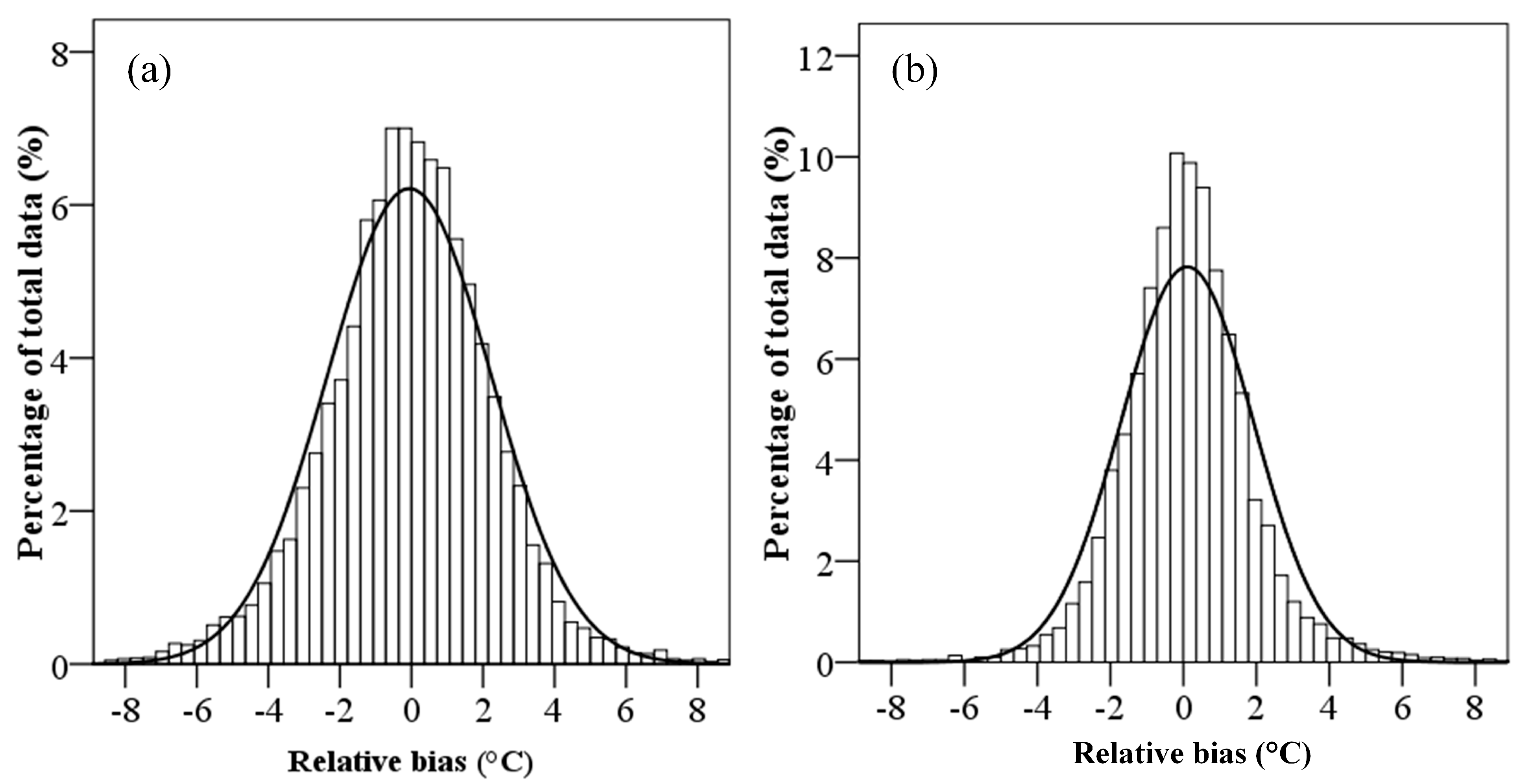
Using the selected models, the frequency distribution of the relative bias between estimated Ta and observed Ta for all three land-cover types is close to the normal distribution curves and almost symmetrical with the mean bias centered in zero (0.01 for Tmax estimation and 0.06 for Tmin estimation). The temperature error ranged between −8 °C and 8 °C (
Figure 2). For Tmax, approximately 38%, 66%, and 83% of all estimations were within 1 °C, 2 °C, and 3 °C absolute bias, respectively. For Tmin, approximately 50%, 79%, and 92% of all estimations were within 1 °C, 2 °C, and 3 °C absolute bias, respectively.
Figure 2.
Relative bias distribution considering all Tmax (a) and Tmin (b) estimations with the selected models in the study area for all the three land-cover types. (The black curves are the normal distribution curves).
Figure 2.
Relative bias distribution considering all Tmax (a) and Tmin (b) estimations with the selected models in the study area for all the three land-cover types. (The black curves are the normal distribution curves).
At the regional scale, the estimation accuracy of both Tmax and Tmin varied with phases of the growing season. For all the three land-cover types (
i.e., crops, forest, and urban), the accuracy of estimated Tmax and Tmin was higher in June, July, and August) than that either in May or September (
Figure 3). Performance was also analyzed for each meteorological station. Results showed that about 83% of the stations had a correlation higher than 0.80, MAE lower than 1.50 °C and RMSEs lower than 2.5 °C for Tmax. By comparison, about 85% of the stations had a correlation higher than 0.88, MAE lower than 1.10 °C and RMSEs lower than 2.0 °C for Tmin. Generally, the stations located in deciduous forest had a better performance than those in crop and developed areas. The spatial distribution of RMSE shows that the majority of the stations with lower performance in Tmax estimation were located in the areas with higher elevation (specifically, east of Nebraska and northwest of Iowa) and in the northeast of Illinois (
Figure 4). The spatial and temporal patterns are discussed in Section 6.2.
Figure 3.
Accuracy of estimated Tmax (a–c) and Tmin (d–f) (RMSE, °C) in different months from 2008 to 2012 over three land-cover types (forest, developed and crop).
Figure 3.
Accuracy of estimated Tmax (a–c) and Tmin (d–f) (RMSE, °C) in different months from 2008 to 2012 over three land-cover types (forest, developed and crop).
Figure 4.
Spatial distribution of Tmax (a) and Tmin (b) (°C) estimation accuracy (RMSE) for all the meteorological stations.
Figure 4.
Spatial distribution of Tmax (a) and Tmin (b) (°C) estimation accuracy (RMSE) for all the meteorological stations.
5.3. Correlation Analysis of MODIS Ts and Tmax
It is interesting that Tmax has stronger agreement with Ts-night than Ts-day. In addition, higher Tmax estimation accuracy was observed with the combination of both Ts-day and Ts-night than with either of them alone. As shown in
Table 2, Ts-day and Tmax have similar correlation coefficient in deciduous forest and developed area, while it is significantly lower in cropland. Fu
et al. [
18] also found that estimation using linear regression of Tmax from MODIS Ts-day was not accurate enough in the growing season (
p > 0.01, R2 < 0.10) compared to the non-growing season (
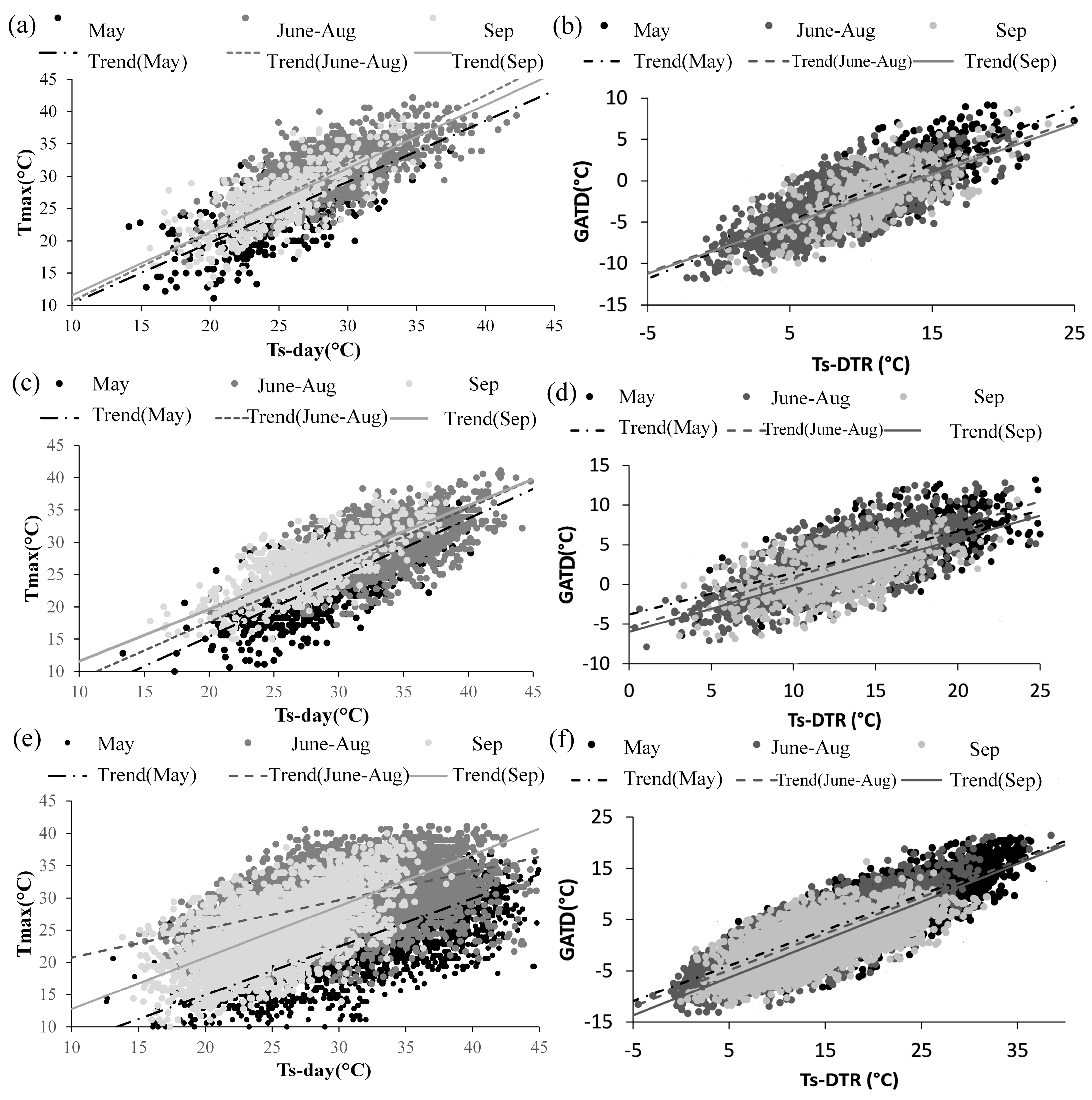
p < 0.01, R2 > 0.40). In cropland areas, the Ts-day and Tmax relations can be varied and complex at different periods during the growing season, as the vegetation cover is changing over time and different crop types are planted in rotations from year to year. As shown in
Figure 5e, compared with
Figure 5a,c notable differences can be observed in Tmax and Ts-day relationship during different phases of the growing season in crop areas. While, it is shown from
Figure 5b,d,f that both GATD and Ts-DTR have similar linear correlation relationships (trend) in different seasons from May to September for all three land-cover types, especially for crops compared to the relation between Ts-day and Tmax.
Figure 5.
Scatterplot of Ts-day vs. Tmax (°C) and GATD vs. Ts-DTR (°C) for: (a,b) forest; (c,d) developed; and (e,f) crops areas across the entire study area from 2008 to 2012.
Figure 5.
Scatterplot of Ts-day vs. Tmax (°C) and GATD vs. Ts-DTR (°C) for: (a,b) forest; (c,d) developed; and (e,f) crops areas across the entire study area from 2008 to 2012.
As at the beginning of the growing season, vegetation fraction is low and the land’s surface is composed primarily of bare soil. Ts-day is usually much higher than Tmax during this period as more energy is partitioned into sensible heat flux from the soil as opposed to later in the year when crops have emerged and are transpiring (latent heat flux) [
41]. During the green-up phase of crops, the spatial coverage of vegetation increases, leading to transpirational cooling, increased latent heat fluxes, decreased sensible heat fluxes, and in general a reduced daytime GATD [
41]. During the senescence phase of crops, as maturity is reached, photosynthesis and transpiration decrease, the latent heat fluxes decreases, the sensible heat fluxes increase resulting in higher GATD [
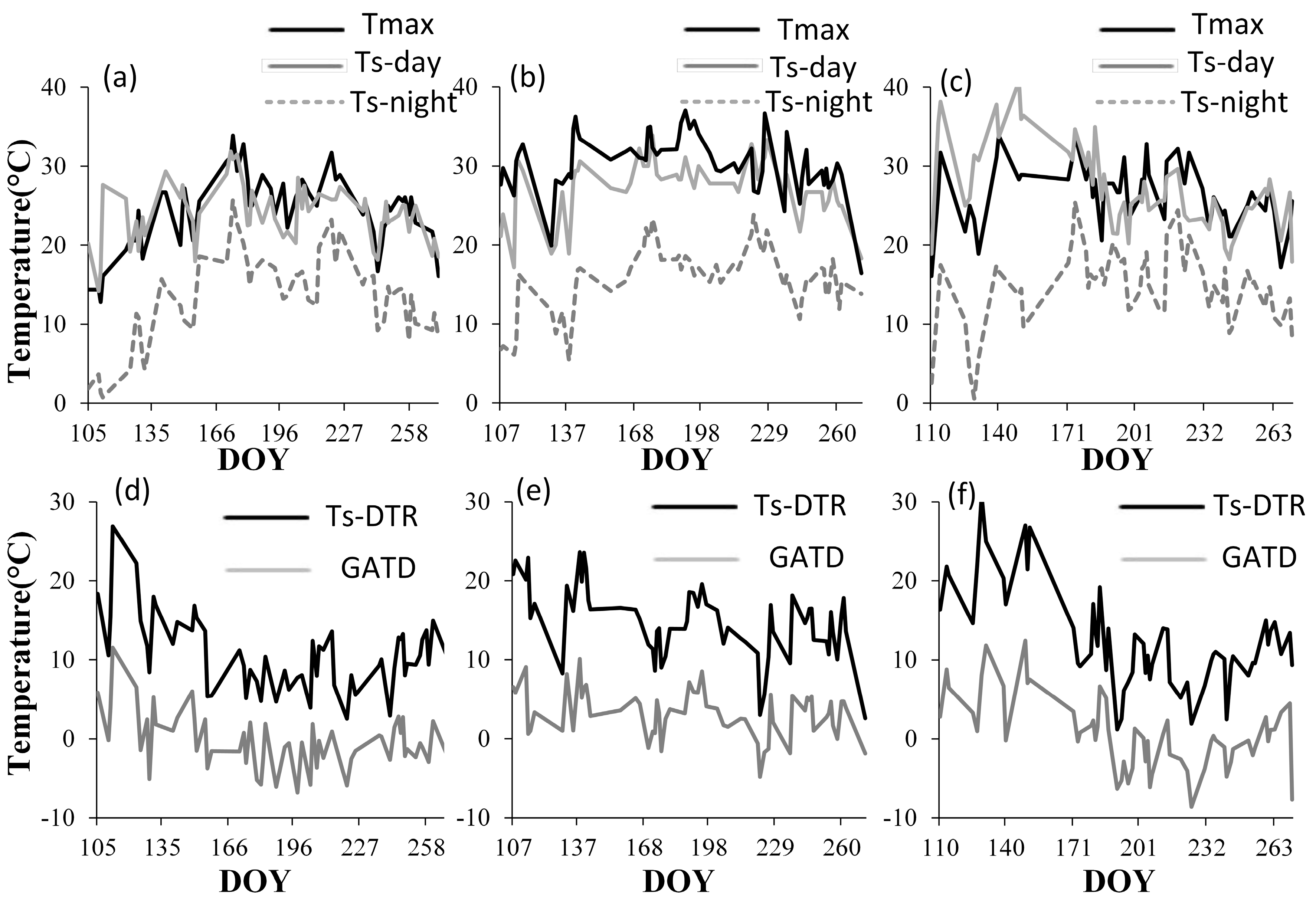
41]. Thus, over crop areas Ts-day is typically much higher than Tmax at the beginning of the growing season, slightly lower than or equal to Tmax in the middle stage of the growing season and slightly higher than or equal to Tmax in the end of the growing seasons (
Figure 6c). While in deciduous forest and developed area, Tmax increases with Ts-day proportionally and the seasonality effect is minimal (
Figure 5a,c,
Figure 6a,b).
Figure 6.
Typical Tmax, Ts-day and Ts-night (°C) curves (a–c), Ts-DTR and GATD (°C) curves (d–f), of three land-cover types: (a,d) deciduous forest (in Albia 3 NNE, 2009); (b,e) developed (in Columbus port Columbus international airport, 2009); and (c,f) crops (in Little Sioux 2 NW, 2009).
Figure 6.
Typical Tmax, Ts-day and Ts-night (°C) curves (a–c), Ts-DTR and GATD (°C) curves (d–f), of three land-cover types: (a,d) deciduous forest (in Albia 3 NNE, 2009); (b,e) developed (in Columbus port Columbus international airport, 2009); and (c,f) crops (in Little Sioux 2 NW, 2009).
As expected, a strong linear relation between GATD and Ts-DTR was observed for all stations from 2008 to 2012 in the study area (
Figure 7). It is the reason why combining Ts-day and Ts-night to estimate Tmax could minimize the influence of these factors and a higher accuracy could be achieved. In the absence of solar radiation, Ts-night is affected by fewer factors and is more stable than Ts-day [
10,
21,
22]. Even with the same solar radiation, the relationship between Ts-day and Tmax is affected by several factors like vegetation changes, land-cover types, soil moisture, precipitation, wind speed,
etc. [
4,
20]. Similarly, with the same solar radiation, the relationship between Ts-day and Ts-night is affected by the abovementioned factors in the same way. Many previous studies have shown that both GATD and Ts-DTR increase with elevation and decrease with increased vegetation cover, cloud cover, soil moisture and precipitation, respectively [
19,
20,
25,
42,
43,
44]. For example, in the developed or low soil moisture areas (e.g., desert), both the DTR and Ts-day can be much higher than that of forest areas or wet areas.
Figure 7.
Scatterplot of Ts-DTR vs. GATD (°C) for all station from 2008 to 2012.
Figure 7.
Scatterplot of Ts-DTR vs. GATD (°C) for all station from 2008 to 2012.
5.4. Spatial and Temporal Patterns
Spatially, relatively lower accuracy was observed in northwestern Iowa, eastern Nebraska and northeastern Illinois (
Figure 4). The spatial and temporal patterns of Tmax agree well with the MIDV patterns during the study period. Similar to the result of Landsberg’s [
38] study, in the Corn Belt, the Tmax IDV showed a spatial zonal pattern (
Figure 8) of increasing with latitude. It was also higher in spring and autumn than summer. The stations with larger Tmax IDV (>2.6) tend to have lower Tmax estimation accuracy (
Figure 4 and
Figure 8). In addition, the correlation coefficient between Tmax MIDV and Tmax RMSE in individual stations during the study period 2008 to 2012 was 0.41 (
p < 0.01) (
Figure 9). On the regional scale, the Tmax MIDV from May to September were 3.51 °C, 2.67 °C, 2.17 °C, 2.12 °C, and 2.99 °C, respectively. It also agrees well with the trends of Tmax estimation accuracy temporally, which is also highest in May and lowest in August. For Tmax estimation, there is a trend that higher Tmax IDV resulted in higher Tmax estimation errors (
Figure 10a,c). The Ts tended to overestimate Tmax if the Ta of the current day was lower than that of the previous or/and next day and to underestimate Tmax if the Ta of the current day was higher than that of the previous or/and next day (
Figure 10a,c). The day-to-day difference of Tmax can reflect the changes of air masses, as well as the sources of air masses and their sources and major paths [
38]. Generally, air is mainly heated by land surface, however air masses usually strike the local energy balance. Cool air moving over a warm surface is heated from below and warm air moving over a cool surface is cooled from below [
45]. There is a time lag for the establishment of new balance between air and land surface temperature. As a result, before that, with cool air and warm air, LST tends to overestimate and underestimate Ta, respectively, when using LST to estimate Ta.
Figure 8.
MIDV of (a) Tmax and (b) Tmin (°C) of the individual stations during 2008–2012 throughout the growing season.
Figure 8.
MIDV of (a) Tmax and (b) Tmin (°C) of the individual stations during 2008–2012 throughout the growing season.
Figure 9.
Scatterplot of Tmax MIDV vs. Tmax RMSE (°C), of all individual stations included in this study during 2008 to 2012.
Figure 9.
Scatterplot of Tmax MIDV vs. Tmax RMSE (°C), of all individual stations included in this study during 2008 to 2012.
Figure 10.
catterplot of estimation error (estimated Ta minus observed Ta) of Tmax (a) and Tmin (b) vs. the IDV of the current day (Equation (3)), and estimation error of Tmax (c) and Tmin (d) vs. the IDV of the next day (Equation (3)), for crop area during 2008–2012 throughout the growing season.
Figure 10.
catterplot of estimation error (estimated Ta minus observed Ta) of Tmax (a) and Tmin (b) vs. the IDV of the current day (Equation (3)), and estimation error of Tmax (c) and Tmin (d) vs. the IDV of the next day (Equation (3)), for crop area during 2008–2012 throughout the growing season.
In addition, irrigation might have contribute to the low Tmax estimation accuracy in eastern Nebraska. The relationship between observed and estimated Tmax in this area was examined and it was found that the Ts of these stations (e.g., Columbus 3 NE, Friend 3 E, and Surprise) that are dominated by irrigated crop land, tends to underestimate the Tmax, especially in 2012, due to irrigation. According to the 2007 Census of Agriculture, of approximately 55 million acres under irrigation nationally, about 15% are located in Nebraska (8.56 million acres) [
46]. About three out of eight cropland acres in Nebraska are under irrigation [
46]. Thus, it is reasonable to expect Ts would underestimate Ta in heavily irrigated landscapes where targeted water applications result in significant cooling effect on the land surface as well as the canopy, as more energy is partitioned to the latent heat flux via evapotranspiration [
41]. The air will be cooled after irrigation as well, but compared to the decrease of Ts value, the decrease of Ta is very small.
As for Tmin estimation, there is no apparent relation spatially. In addition, there is no obvious relation between Tmin IDV and Tmin estimation errors (
Figure 10b,d). Landsberg [
38] stated that, as compared to changes in Tmax, changes in the Tmin are less affected by air masses but much more affected by local conditions such as proximity to water bodies and mountains orographic tendencies for inversion formation, and other environmental characteristics. This may be a possible reason for the low accuracy in Tmin estimation in northwestern Iowa. While at a regional scale, the trends of Tmin MIDV from May to September (2.75 °C, 2.24 °C, 1.87 °C, 2.10 °C, and 2.60 °C, respectively) agree well with that of Tmin estimation accuracy (
Figure 3).
There may also be some other possible reasons leading to the low estimation accuracy. Though combining both Ts-day and Ts-night to estimate Tmax reduced the impact of land-cover types and vegetation cover changes, vegetation variables might still have impact on the Ta estimation accuracy. It is shown from
Table 2 that by integrating DOY information, the estimation accuracy of models for both Tmax and Tmin were improved, especially in crops areas and forest areas. As vegetation had been variously contributed to latent heat flux, canopy resistance to transpiration [
19]. DOY included the information of vegetation cover changes with seasons. Remaining clouds (pixel and sub-pixel) negatively affect the model performance. Though only pixels marked as cloud-free were selected and the cloud cover of the 13-by-13 pixel window was less than 10%, there were still some cloud-contaminated pixels included. Thin or sub-pixel cloud cover detection is difficult [
47] and the LST retrieved under these conditions often corresponds to top-of-cloud temperature [
4,
48]. In addition, most undetected cloud-contaminated LST outliers occur in cloud edges and a large proportion of the pixels with higher errors occurred near identified clouds [
33,
49]. However, cloud-edge elimination, such as considering a 10-km buffer [
48], could limit data availability significantly. Thus, some errors and uncertainty have been brought into this study by cloud contamination in order to collect a sufficient sample size of pixels. Other factors could also explain some of the errors in Ta estimation from Ts. Prihodko and Goward [
19] observed deviations of 0.6 °C at horizontal distances of 6-km from a dense spatial ground network of meteorological stations. The temperature in the 13-by-13 windows is quite homogeneous in flat terrain conditions. However, temperature may show larger spatial variations in hilly areas (e.g., the northwest of Iowa) [
22].


 ,
, 


