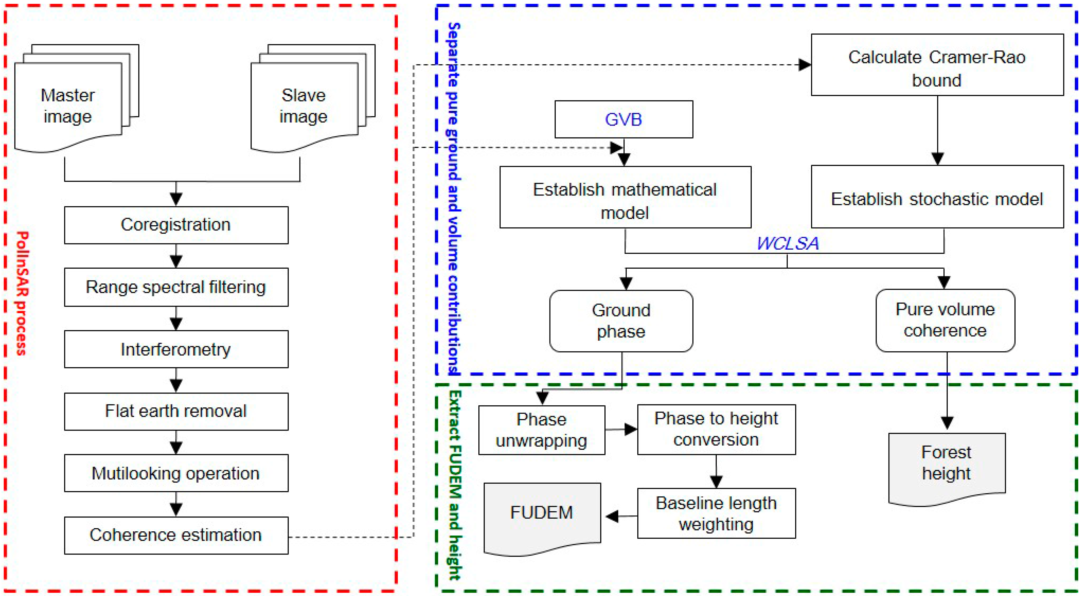
3.1.1. Mathematical Formulation
When considering a data-set constituted by
m baselines PolInSAR data. We synthesize
n interferometric coherence values by varying the polarization
[
1,
5]. Thus, each coherence can be expressed as
where
k = 1, 2, 3,
,
m and
j = 1, 2, 3,
,
n.
f represents the scattering model as given in Equation (4). Since the level of the temporal decorrelation is usually unknown, it is not possible to express all the ground phase with a ground height and vertical wavenumber
[
16,
18]. Therefore, the ground phase
is estimated separately for every baseline in this paper. The GVR
is assumed to be constant between interferometric pairs in the same polarization. This is suitable for all interferometric pairs performed at common band, with similar incidence angles and under similar weather condition [
18]. Moreover, considering the high complexity of Equation (3),
is parameterized by
. Starting that every baseline has a distinct pure volume coherence
caused by distinct
. Then, Equation (6) can be rewritten as
Thus, before extracting the forest height and FUDEM, first we can separate the pure ground and volume contributions by estimating and . Note that, in this scheme, there are three forest parameters , which can only be inverted if at least two different PVCs are provided. In other words, we must provide at least two different interferometric pairs to invert the forest parameters.
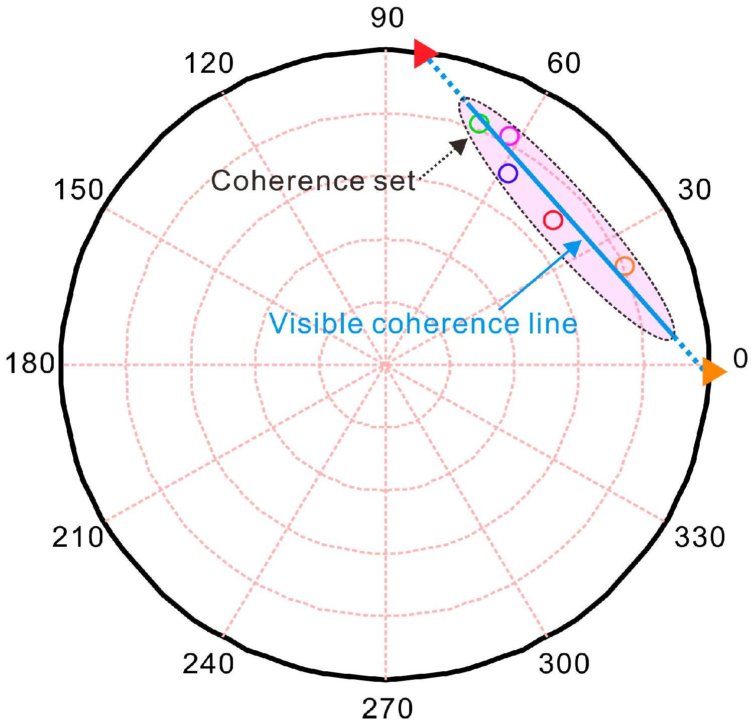
As to the choice of
n polarizations, in order to ensure that NRO ≥ 0, at least two polarizations (
n ≥ 2) must be provided to obviate the rank defect of Equation (7). Furthermore, we suggest that the selected
n polarizations should have distinct GVRs. The reason is that polarizations with distinct GVRs are helpful to form a well-conditioned inversion of Equation (7). For this purpose, optimum states [
1] can be selected to produce a sample set in a coherence region since they tend to find the boundary revealing the shape of a coherence region [
28]. As a result, compared to Pauli and linear polarizations [
1], a longer visible coherence line can be observed by optimum states, which enables the estimation to be robust against the effect of coherence noise. Moreover, although increasing the number of polarizations cannot provide more redundant observations to estimate the forest parameters
, it can reduce the effect of gross error in some observation on the estimations and allow us to enhance the reliability of ground phase and PVC.
3.1.2. Stochastic Model
Because the ground is strongly polarization-dependent, different polarimetric interferograms may be perturbed by different levels of noise [
1,
2]. Moreover, different interferometric pairs are also perturbed by different levels of noise caused by the wind-induced temporal decorrelation [
29,
30,
31].
In order to model the contributions of observation errors to the estimations, empirical errors of the observations [
4] and the COMENT method [
16] have been used to estimate the covariance matrix of the observations. In this paper, the Cramer–Rao bound [
1,
21] is used to calculate variances of the observations and a diagonal covariance matrix can be formulated with assuming the observation errors are uncorrelated. The Cramer–Rao bound on variance of coherence magnitude can be approximately related to the coherence as [
1,
21]
where
N is the number of independent samples used to estimate the coherence. Next, we adjust the contributions of the different interferometric coherences through
. The higher the interferometric coherence, the smaller the variance, and the larger the weight. The corresponding expression is
where
is the weight associated with the interferometric coherence of
.
3.1.3. Parameter Estimation
The complex least squares [
32] can preserve many of the original attributes of the interferometric coherences, while reducing the disturbance of the observation errors. This approach has been widely used in model-based PolInSAR and SAR tomography inversion procedures [
2,
4,
33,
34,
35]. Based on the complex least squares, the inversion algorithm for Equation (7) can be formulated as
where
is the observation measured by PolInSAR.
H represents the complex conjugate transpose.
represents the weight of observation
and can be estimated by Equation (9). For estimation scenario like Equation (10), non-linear least squares has been widely adopted to enumerate the unknown parameters [
2,
17,
18]. In fact, such problem can also be regarded as a surveying adjustment problem, which has been widely discussed in geodesy and various theories and methods have been developed to study the relationship between observation errors and unknown parameters [
36]. However, the existing adjustment methods are mainly designed for real number. Therefore, in this paper, we will introduce how to solve Equation (10) with an adjustment method.
For non-linear inversion of Equation (10), one widely used approach is the linearized strategy based on the Taylor series which is adopted to expand the nonlinear function as an approximate linear function [
36]. Although this expansion is valid for complex function, we should keep in mind that
in Equation (7) is a complex and we should make a discussion about the stringent mathematical condition imposed on the complex differentiation [
32]. In order to overcome this limitation, an alternative way to avoid complex derivative is the complex
can be regarded as being composed of two real parameters
a and
b. In such way,
f can be reconstructed with two real functions to express the real and imagery parts. Lastly, Equation (7) can be rewritten as
where
represents the derivative operation and
,
,
, and
are the corrections of the approximations of unknown parameters.
and
are the differences of the real and imaginary parts between observations and model predicted values. Matrix notation is used to express Equation (11) as follows
Actually, from Equation (12), we can conclude that Equation (10) is equal to a combined adjustment of complex real and imaginary parts. In addition, the weight
in Equation (10) accounts for the noise contribution of a complex coherence, which is equal to set the common weight for the real and imaginary parts in Equation (12). In such way, the complex least squares in Equation (10) is converted to a least squares of real case and we can extend the surveying adjustment method into such inversion. The WCLS solution can be obtained directly from Equation (12) [
36]
However, we find matrix
B in Equation (13) is sparse and ill-conditioned, which results in an unstable estimation of
. The Butterworth singular value decomposition (B-SVD) [
37] is applied to estimate
in order to overcome the above-mentioned limitation. By B-SVD, the
can be estimated with
where
is the Moore–Penrose inverse of
and
D is the Cholesky decomposition of
W−1. We recommend using iterative WCLS to calculate the unknown parameters because the start values are just initial guesses. To provide the start value as accurate as possible, a simple but well-defined approach described by Equations (8.47–8.50) in [
1] is recommend to calculate the initial values. If we have other reliable constraint conditions about the domain of the unknown parameters, these can also be easily embedded into Equation (12a) to enhance the inversion procedure [
36,
38]. Thus, we complete the GVB model inversion procedure with the WCLSA method.


