1. Introduction
Rice is recognized as one of the most important crops in the world and the staple food for more than half of the world’s population [
1]. Leaf Area Index (LAI) is defined as one-half the total green leaf area per unit of ground surface area [
2], and the total weight of plant parts above the ground per unit area at any particular time is called the aboveground biomass (AGB). LAI and AGB are both important vegetation biophysical variables that are widely applied in crop growth monitoring and yield estimation [
3]. Timely acquisition of crop information on LAI and AGB is vital for the design of dynamic maps of rice growth parameters. Such data could support agronomic decisions that ensure plant health, yield stability, and optimization of economic benefits.
Traditional crop growth monitoring methods are limited in space and time, especially in meeting the requirements of continuous crop condition monitoring at regional scales. Remote sensing techniques offer a feasible tool for parameter regionalization. Lu made a review of the potential and challenge of remote sensing-based forest biomass estimation; Koppe et al. did a study on the estimation of winter wheat biomass using 30 m resolution data from Hyperion on regional scale; and Liu et al. explored the uncertainties in green LAI estimation from Landsat images over multiple growing seasons with several crop types [
4,
5,
6]. However, few studies have been conducted on the dynamic map** of crop growth parameters, which is important for practical applications. Currently, the most widely used method for estimating LAI or AGB of crops from remote sensing data is through the use of statistical relationships between the parameters and spectral vegetation indices (VIs) derived from many different kinds of optical remote sensing data [
7,
8,
9] or other nonparametric methods [
10,
11]. Some researchers have explored the physical model inversion methods with satisfactory results [
10,
12]. These inversion models usually contain many parameters and often require extensive details of meteorological and/or agricultural knowledge to run, making real-time inversion on a regional scale unsuitable. However, less is known about the application of machine learning methods and their potentials in inverting crop biophysical parameters using remote sensing data.
The Advanced Very High Resolution Radiometer (AVHRR), Moderate Resolution Imaging Spectroradiometer (MODIS), Satellite pour l’Observation de la Terre VEGETATION (SPOT-VGT) and Landsat-MSS have demonstrated advantages in rice monitoring from regional to global scales due to wider coverage and relatively longer data archive [
13,
14,
15]. Some coarse resolution data such as AVHRR-NDVI, MODIS-NDVI, and MODIS-EVI have been preprocessed and provide standard VI products at a global scale to end users [
16,
17,
18]. However, coarse resolution satellite data are generally prone to classification uncertainties as mixed land cover types are difficult to delineate, especially in the highly fragmented rice fields in the eastern plains of China [
19]. Moreover, in practice, crop LAI was found to be significantly underestimated by the MODIS LAI product [
20,
21], which makes the implementation of suitable field management practices at a local scale more complicated.
Middle to high spatial resolution satellite data, e.g., Landsat TM/ETM+/OLI, SPOT and China Brazil Earth Resources Satellite (CBERS), are promising in capturing small patches of crop fields [
22]. However, their cost and relatively long revisit cycles partially offset their advantages in spatial resolution. Specifically, most of the rice fields located in the subtropical regions of China are influenced by the monsoon climate, leading to inadequate acquisitions of cloud-free remote sensing data during monsoon weather conditions. In precision agriculture, where rice growth information is critically needed, high-resolution multi-temporal remote sensing data are advantageous, as the spatial variability captured by remote sensing data is useful for adjusting crop properties while taking into account the local conditions [
5].
Two small environment and disaster monitoring and forecasting satellites (HJ-1A/B) were launched by the China Center for Resources Satellite Data and Applications (CRESDA) in 2008. The charge-coupled device (CCD) cameras of these satellites have a swath width of 700 km, four spectral bands with a spatial resolution of 30 m in the visible bands, and a revisit cycle of four days (the revisit cycle of the constellation is two days). This fine spatial resolution and short repeat cycle facilitate the availability of images at all critical growth stages of crops [
23,
24].
Vegetation Indices (VIs) are robust empirical measures of vegetation activity at the land surface. They are designed to enhance the vegetation signal from measured spectral responses by combining two (or more) different wavebands, often in the red (0.6–0.7 µm) and NIR wavelengths (0.7–1.1 µm), and are widely used in the studies of crop land classification, yield prediction, phenology, and crop growth monitoring [
25,
26,
27]. The normalized difference vegetation index (NDVI) [
28] is by far the most widely used index in the literature, and is advantageous for studying historical changes; however, it is sensitive to canopy background variations and saturates in relatively high-vegetated areas [
29,
30]. The enhanced vegetation index (EVI) [
30] and the two-band enhanced vegetation index (EVI2) [
31] differ from NDVI by attempting to correct for atmospheric and background perturbation, and appear to be superior in discriminating subtle differences in areas of high vegetation density [
32]. Cumulative VIs have been proven as a surrogate for absorbed photosynthetically active radiation (APAR), which is proportional to total biomass [
33,
34].
The objectives of this study were to evaluate the use of vegetation indices for continuous rice growth monitoring over multiple years and at a regional scale using a newly constructed HJ-1 CCD 10-day composite data, explore the traditional statistical models and nonparametric methods for LAI and AGB retrieval based on extensive field campaign datasets, and propose a dynamic map** method for rice growth for in situ application in agricultural practice.
2. Materials and Methods
2.1. Study Site
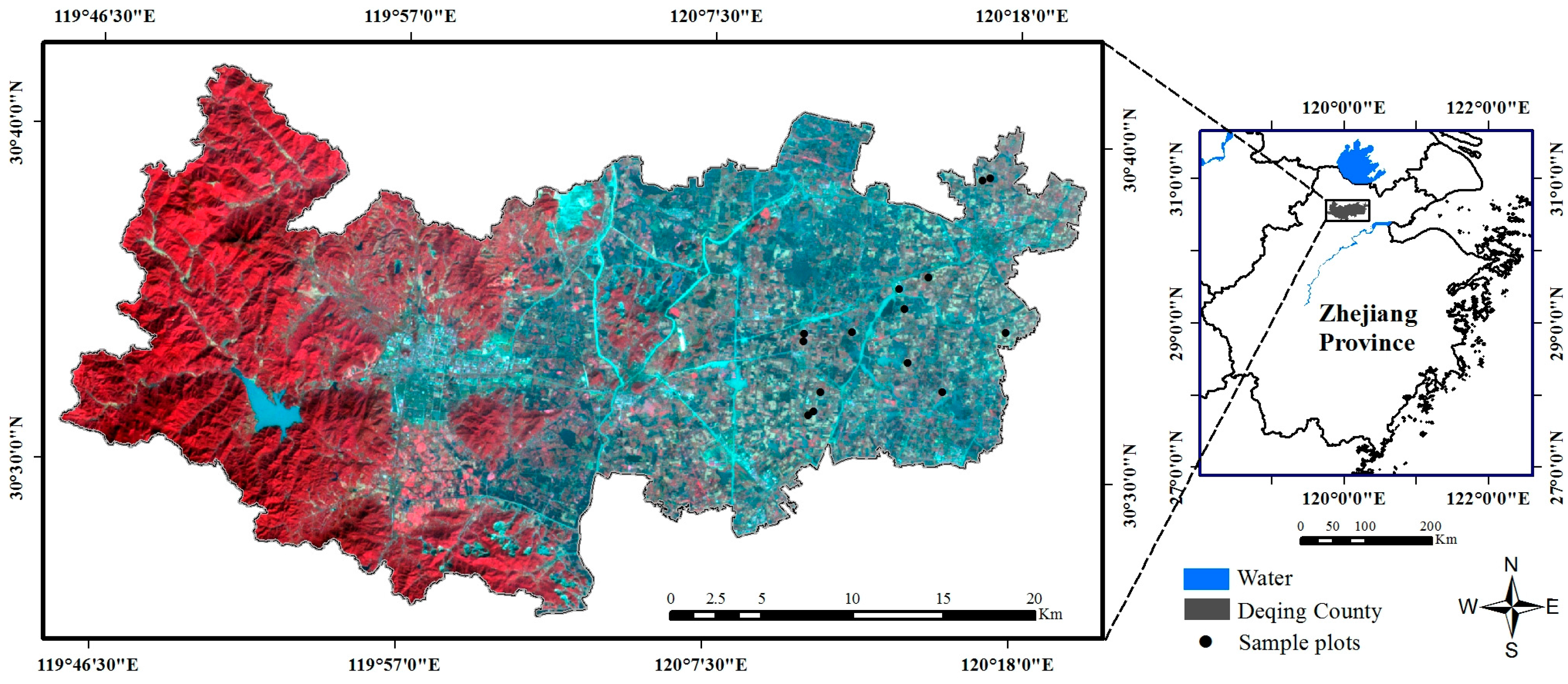
The study was conducted in Deqing County, which lies in the western part of the Hangjiahu Plain, Zhejiang Province, Southeast China (
Figure 1). This area is characterized by a tropical monsoon climate. The mean annual temperature ranges between 13 °C and 16 °C and there is an annual total precipitation of 1379 mm. Deqing has a total area of 936 km
2, and according to statistical data from the local agriculture department, more than 91% of the crop area is single-cropped rice (SCR). However, due to the countless lakes, ponds, and rivers scattered throughout this region, and the well-developed road networks, an irregular crop land phenomenon is typical in the study area [
19].
2.2. Measurement of Crop Parameters
Single-cropped rice is the most abundant crop in Deqing County. Most small patches of rice fields were cultivated by small-scale individual farmers, whereas relatively larger fields were managed by large-scale rice farmers, leading to time inconsistency in rice cultivation and management measures, including different transplanting dates and different rice varieties. Extensive crop parameters experiments were conducted during the rice growing seasons (June to November) for the years 2012 and 2013. Field and laboratory measurements included LAI, AGB, and plant density. The corresponding rice phenology dates and sample numbers for each date were recorded as well (
Table 1).
Rice is cultivated on flooded soils. At the early stages of growth, rice fields are a mixture of green rice plants and open water [
35]. Water depth generally varies from 2 to 15 cm. As rice continues to grow, new leaves emerge. The development of tillers is slow at first and becomes faster until the maximum tiller number is attained at the highest plant density. About 50 to 60 days after transplanting or sowing (the transplanting or sowing dates for 2012 and 2013 were 21 June and 18 June, respectively), rice plant canopies cover most of the soil area. The leaves continue to increase in total area and generally remain green until the heading stage. Due to intraspecific competition at the reproductive stage, the tiller number drops and the rice leaves gradually become yellow. This stage is also associated with an increase in the dry aboveground biomass of rice until maturity (
Figure 2) [
36].
Fourteen rice sample plots with areas larger than 200 × 200 m
2 in Deqing County were randomly chosen in order to measure the vegetation characteristics (
Figure 1). A handheld global positioning system (GPS) receiver (Trimble Juno-SB, Trimble Navigation Ltd., Sunnyvale, CA, USA) was used to record the precise location and geometry of every sample plot with a positioning accuracy of approximately ±5 m. At every measurement time, five quadrants of 0.5 m × 0.5 m were selected from each plot, and all single-cropped plants within selected quadrants were harvested (
Figure 3).
The aboveground parts of rice plants were separated into leaves, stems, and ear (after ear differentiation) in the lab. The leaf areas of single-cropped rice were measured using a leaf area meter (LI-3000C, with conveyor belt assembly, LI-3050C; Li-Cor, Inc., Lincoln, NE, USA). All plant parts were weighted by an electronic scale in fresh conditions at first. Then they were put into the oven at 105 °C for 30 min and kept at 70 °C for 72 h until they reached constant weight. The dry aboveground biomass was weighted with the same electronic balance and scaled to total dry AGB m2 using plant density, which was measured as the average number of plants of five quadrats in each sample plot. The average LAI and AGB of five quadrats in each rice sample plot represent the vegetation characteristic values of that sample plot.
2.3. Remote Sensing Data and Vegetation Indices (VIs)
HJ-1 CCD data from June to November in 2012 and 2013 over the study area were downloaded from the China Centre for Resources Satellite Data and Application (CRESDA). The sensor characteristics are presented in
Table 2. A total of 100 scenes of HJ-1A/B images (46 scenes and 54 scenes in 2012 and 2013, respectively) with cloud cover less than 20% during the single-cropped rice phenology in the study area were selected for the following procedures. All the images collected were processed through radiometric calibration, atmospheric correction, and geometric correction. The formulas and coefficients for radiometric calibration were collected from the raw image package. The atmospheric correction was performed using the Moderate Resolution Transmission (MODTRAN) 4 model integrated in the Fast Line-of-sight Atmospheric Analysis of Spectral Hypercubes (FLAASH) module in the Environment for Visualizing Images (ENVI) package. The images were co-registered using the Second National Soil Survey Vector Map (scale 1:10,000) provided by the Deqing County Land and Resources Bureau, and the geometric accuracy was less than 0.5 pixel (15 m).
Only cloud-free images that corresponded to each field campaign date within three days were selected for LAI modeling. Using Savitzky-Golay (S-G) filters, daily VI time series were created from all the HJ-1 CCD images (100 scenes in two years). These images were used to verify the AGB estimation before dynamic map** [
23,
37]. After modeling and model validation, all of the images were processed with cloud detection and maximum-value composite (MVC) methods to produce a new HJ-1 CCD 10-day composite data for use in the timely dynamic map** of rice growth. Cloud-free pixels usually have lower reflectances between 0 and 0.3 in the red band, whereas thick cloud-contaminated pixels have higher reflectances distributed over large ranges between 0 and 1.7 [
38]. The threshold value for HJ-1 CCD data was selected as 0.25 for the red band after statistics calculated from 1214 cloud pixels and 1029 cloud-free pixels randomly selected from HJ-1 CCD images. The flagged cloudy pixels were set to no data. MVC was initially developed for AVHRR and MODIS VIs data and has been widely used to minimize atmospheric effects, including residual clouds [
39,
40]. MVC was designed based on the assumption that observations with a higher component of haze or cloud will show a higher reflectance in the red band, thus a lower VI value to distinguish the edge between land and residual cloud [
38,
41]. For modeling of LAI from HJ-1 CCD, there were 191 matching LAI sample sites and 194 matching AGB sample sites.
In addition to the selected VIs, NDVI, and EVI2, cumulative VIs were adopted for the estimation of AGB.
The matched cumulative VIs were calculated from day of year (DOY) 173 and 169 for 2012 and 2013, respectively, approximately representing the transplanting date or sowing date of SCR.
2.4. Deriving LAI and AGB via VIs
Pixel-based VI values from the corresponding HJ-1 CCD images at the 10 field measurement plots were extracted from the images. As the SCR LAI drops after heading, the growth stages of SCR were divided into before heading and after heading in order to improve the estimation results.
Best fit linear and non-linear relationships among VIs, LAI, and AGB were established first. In addition to the five traditional regression equations (linear, exponential, power, logarithmic, and quadratic polynomial regression), two machine learning methods, i.e., a back propagation neural network (BPNN) and a support vector machine (SVM), were applied in model construction. The neural network approach has the advantages of nonlinearity, input–output map**, adaptivity, generalization, and fault tolerance [
27]. A SVM for regression analysis is accomplished by solving a convex optimization problem, more specifically a quadratic programming problem [
42]. BPNN and SVM have demonstrated their abilities in dealing with complicated datasets in many fields like classification [
43,
44] and data mining [
45,
46].
In this work, the neural network function in the MATLAB package was used for the BPNN regression; LIBSVM 3.20 [
47] and LIBSVM-FarutoUltimate toolboxes (software available at
http://www.ilovematlab.cn) were used for the SVM analyses. The kernel function used in SVM was the radial basis function (RBF) kernel [
42]. The two tuning parameters used in the RBF kernel for LIBSVM are “cost” (C) and “gamma” (γ). The ranges of γ and C were set to [–15, 15] and [–15, 15] for regression, and the steps were 0.5 and 0.5, respectively. To find the optimal parameter, an iterative grid search was applied in which the evaluation was provided by a 10-fold cross-validation for both BPNN and SVM regression.
The leave-one-out cross-validation (LOO-CV) method was implemented to test the prediction capability of the models. This method sets a single observation from the original sample as validation data, and the remaining observations as training data. The performances of the models mentioned above were compared on the basis of cross-validation coefficient of determination (
) and relative cross-validation root mean square error (
RRMSECV).
RRMSECV facilitates comparison of the accuracy of each estimation model and was calculated using the following equation:
where
n is the number of samples and
and
are the predicted and observed values, respectively.
is the observed mean value. All analyses were conducted in the MATLAB program environment.
Furthermore, we verified the relationship between the 10-day composite VI data with AGB. The AGB curve can be described with logistic curves [
36]; the particular form of the logistic equation available was written as:
where
W is the dry aboveground biomass weight of the crop,
t is time,
k is the growth rate,
A + C is the maximum theoretical AGB weight, and
b is a constant term. The accuracy of the model result was determined by
R2 and was accomplished using the MATLAB program. The cumulative VIs were calculated from all 10-day composite data and the corresponding AGB values were estimated from the aforementioned logistic function. The relationships between daily cumulative VIs and 10-day composite cumulative VIs were analyzed, and the best regression equation was built for the dynamic map** application.
2.5. Dynamic Map**
The spatial distribution and temporal dynamics of LAI and AGB of SCR were determined using the best regression model based on the HJ-1 CCD 10-day composite data during the SCR growth season. Before the dynamic map** process, the planting area of single-cropped rice was estimated using a stepwise classification strategy proposed by Wang et al. [
19]. The total acreage of the single-cropped rice was about 94.0 km
2. The levels of SCR growth parameters were visualized with different colors.
4. Discussion
The LAI remote sensing products now available are usually of coarse spatial resolution and LAI values have mostly been underestimated due to the mixed-pixel problem [
48]. Little research has been done on the remote sensing of rice AGB at higher spatio-temporal scales and multi-season dynamic map** of the entire growth process. Considering the growing importance of biophysical parameters in sha** local agronomic activities, there is an increasing need for the precise monitoring of rice crop growth conditions, especially in the eastern plains region of China, where rice fields are relatively irregular and fragmented. The current study is focused on the near-real-time dynamic map** of rice growth using multi-temporal middle- to high-resolution remote sensing time series data for regional-scale applications. A comprehensive field campaign was carried out to record the growth parameters of single-cropped rice, including LAI, AGB, and plant density, and was used in model construction and verification. VIs were derived from HJ-1 CCD images for the purpose of growth parameters inversion.
Time series NDVI and EVI2 were calculated from HJ-1 CCD images, which corresponded to the field campaigns within three days. Vegetation indices combined with reflectance bands showed a high correlation with LAI and AGB (
Table 3). VIs have the advantage of obtaining relevant information rapidly and easily, and perform better than a single spectral band in crop monitoring [
24,
49,
50]. In situ measured LAI reached a maximum, while in situ measured dry AGB continued to increase, and the AGB includes more photosynthetically inactive components (e.g., stem, ear) than the leaf area, which is likely to affect the relationship between VIs and the photosynthetically active components [
34]. In this situation, cumulative VIs were proposed as a better approach for the estimation of AGB.
The regression model chosen for the derivation of SCR growth parameters is another important issue in model construction. The traditional models (linear, exponential, power, logarithm, and quadratic polynomial regression) are commonly used in crop LAI and dry AGB estimation in previous studies [
25,
51]. Partial least squares regression and stepwise multiple regression models have been tested as feasible tools in information extraction [
52], but at the same time introduce a lot of features into the model that result in difficulties in application. There is increasing interest in data mining technology in remote sensing, which is considered to be a useful tool to unravel the non-linear relationship between canopy spectral reflectance and crop growth conditions [
11,
42]. However, few studies have been performed on the application of the technology in agriculture. Backpropagation neural networks (BPNN) and support vector machines (SVM) were applied in model construction in our research. We found that BPNN and SVM performed better than the traditional models in LAI estimation, demonstrating that machine learning methods are potentially useful to understand and predict optical interactions over a wide range of rice canopy LAI. Although the quadratic polynomial regression showed good performance in AGB estimation, the BPNN and SVM methods can also reach comparably high accuracy. This demonstrates that the non-linear methods are efficient in establishing relationships between remote sensing data and rice biophysical parameters.
Most previous studies laid emphasis on rice growth parameters at a single stage, lacking the exploration of consistent growth stages [
53,
54], and, hence, growth monitoring systems were difficult to find in practice. In order to improve the regression precision, we made use of the specific growth curve of SCR. After the heading stage, as LAI drops due to etiolation and senescence of the leaves, the whole growth period was divided into before heading and after heading stages. The accuracy of LAI estimation was improved with this strategy. EVI2 had better results at the before heading stage than NDVI. This may be caused by the saturation of NDVI in relatively low-vegetated areas; this result agrees with that of Shang et al. [
51], who also showed that EVI2 was more resistant to saturation at high biomass range than NDVI.
The cloudy pixels were flagged by a threshold value of 0.25 for the red band of HJ-1 CCD data. The MVC method can further help in the removal of contaminated pixels [
55,
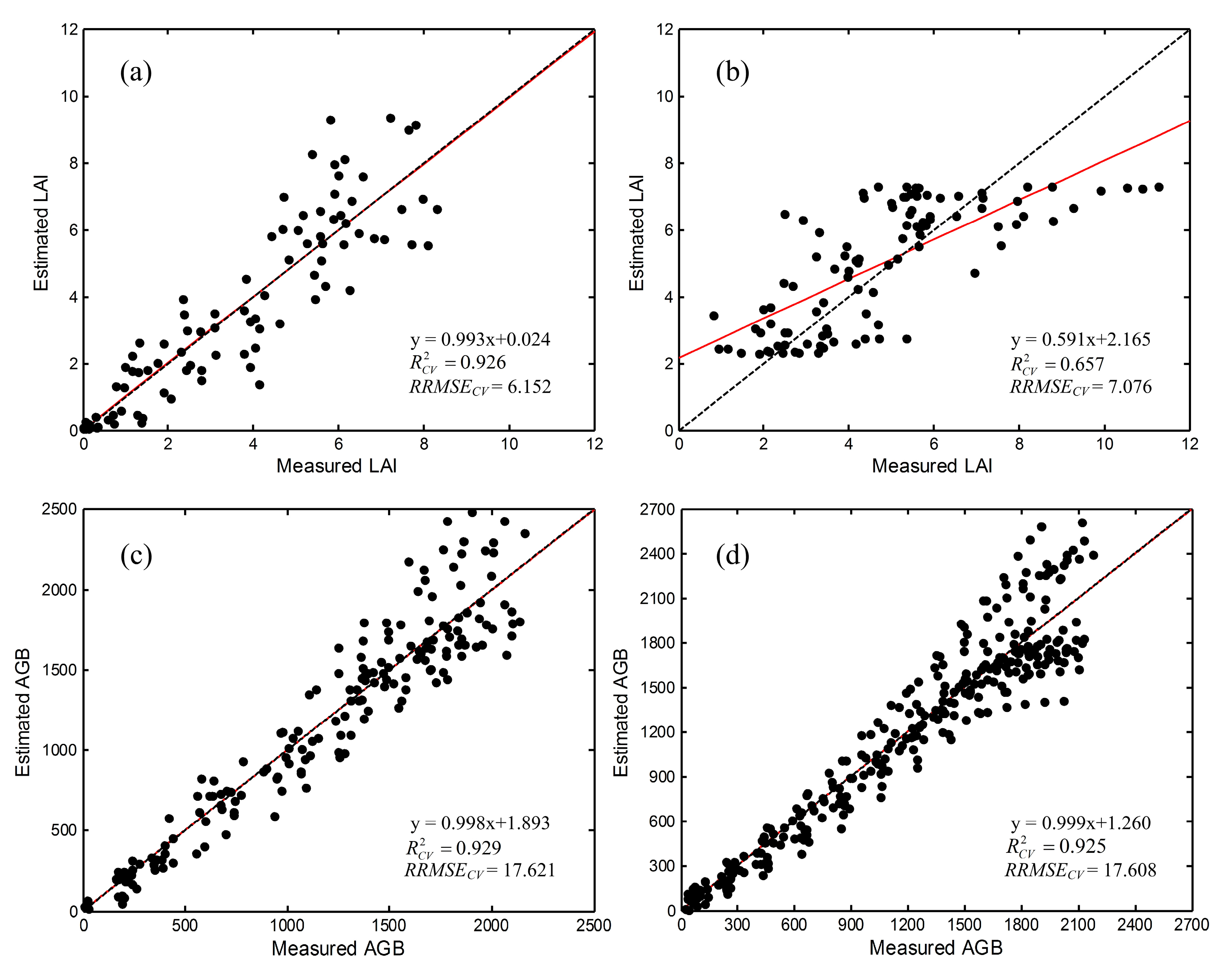
56]. New 10-day composite HJ-1 CCD data were then acquired three times a month for estimating local SCR growth parameters. In the rice growth monitoring and dynamic map** system, EVI2-BPNN regression is selected for before heading LAI estimation; NDVI-SVM is selected for after heading LAI estimation; cumulative NDVI based on the quadratic polynomial fit function was adopted for the all-stage AGB prediction. The
values were 0.93, 0.66, and 0.93, respectively. With this method, rice growth conditions can be visually captured at the regional scale, which will help users compare the overall condition of crops through different growth stages within one year or different years in the same growth stage.
However, it should be noted that the empirical equations built between remote sensing derived VIs and rice growth parameters were partially determined by field experiment data and remote sensing image preprocessing. As the rice planting area may change annually, precise extraction of the crop planting area is crucial for the map** of growth parameters. There are, therefore, inevitable uncertainties in estimation accuracy. When extrapolating this dynamic map** system to other regions, considering the variations in field experiment methods and remote sensing data characteristics, necessary verification steps must be taken. According to Koppe et al. and ** et al., TerraSAR-X (Germany) data and RADARSAR-2 (Canada) data have been successfully used in crop monitoring [
54,
57]. Synthetic aperture radars (SARs) have some advantages for monitoring crop growth status as they are not influenced by the presence of clouds or haze. However, SAR images are usually limited by image processing techniques [
25]. The method proposed in this research made full use of HJ-1 CCD images with high temporal resolution, acquired concurrently with the field data. Considering that HJ-1 data mostly cover China and some surrounding Asian countries and not the whole globe, the sensors only have four wavebands (
Table 2); future studies should be directed towards exploring the potential of SAR (Sentinel-1, ENVISAT-ASAR, RADARSAT-1, etc.) and optical remote sensing data (Gaofen series satellite, FORMOSAT-2, Landsat 8, etc.) for monitoring rice growth parameters other than LAI and AGB.
5. Conclusions
In this study, we proposed a dynamic map** method for single-cropped rice growth parameters at regional, annual, and inter-annual scales. The method was developed based on field campaigns conducted in two consecutive rice growing seasons (2012 and 2013), each spanning June to November in Deqing County, Southeast China. Ten-day HJ-1 CCD image composites, giving a total of three image composites per month, were generated for growth parameters retrieval. The field measurements included leaf area index (LAI), aboveground biomass (AGB), and plant density, and were strictly controlled during measurement. The LAI empirical equations were established by dividing the whole SCR growth period into before heading and after heading stages. EVI2 performed better at the fast growth stage (before heading) whereas NDVI showed better accuracy at the after heading stage (relatively slower growth). Two machine learning methods, i.e., backpropagation neural network (BPNN) and support vector machine (SVM), were applied in LAI model construction. Cumulative VIs were proven suitable for the estimation of AGB. Cumulative NDVI based on the quadratic polynomial fit function was adopted for the all-stage AGB prediction.
This study demonstrated the potential of using HJ-1 CCD images in rice growth monitoring. Machine learning methods provided a useful exploratory tool for improvement in the relationships between different combinations of reflectance and crop variables. Much work remains to be done to scale these growth condition estimation relationships across a variety of canopies, and more sources of remote sensing data should be included in the system. Only then will the approach gain sufficient robustness and reliability to be applied at larger scales of agricultural remote sensing.


