3.2.1. Features for Cloud Detection
The red, green, blue (RGB) color model works well for thick cloud detection, but is not as effective in detecting thin clouds and cirrus clouds. The HIS color model, which follows the human visual perception closely, separates the color components in terms of hue (H), intensity (I) and saturation (S). RGB can be transformed to HIS as follows:
where I
, S
, and H correspond to the intensity-equivalent, saturation-equivalent, and hue-equivalent components, respectively.
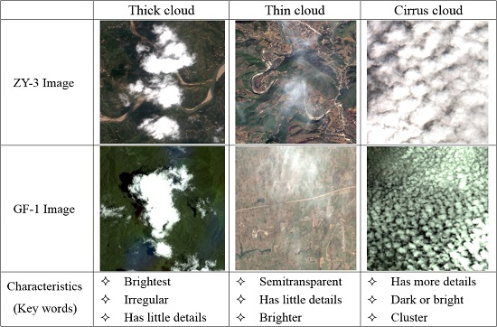
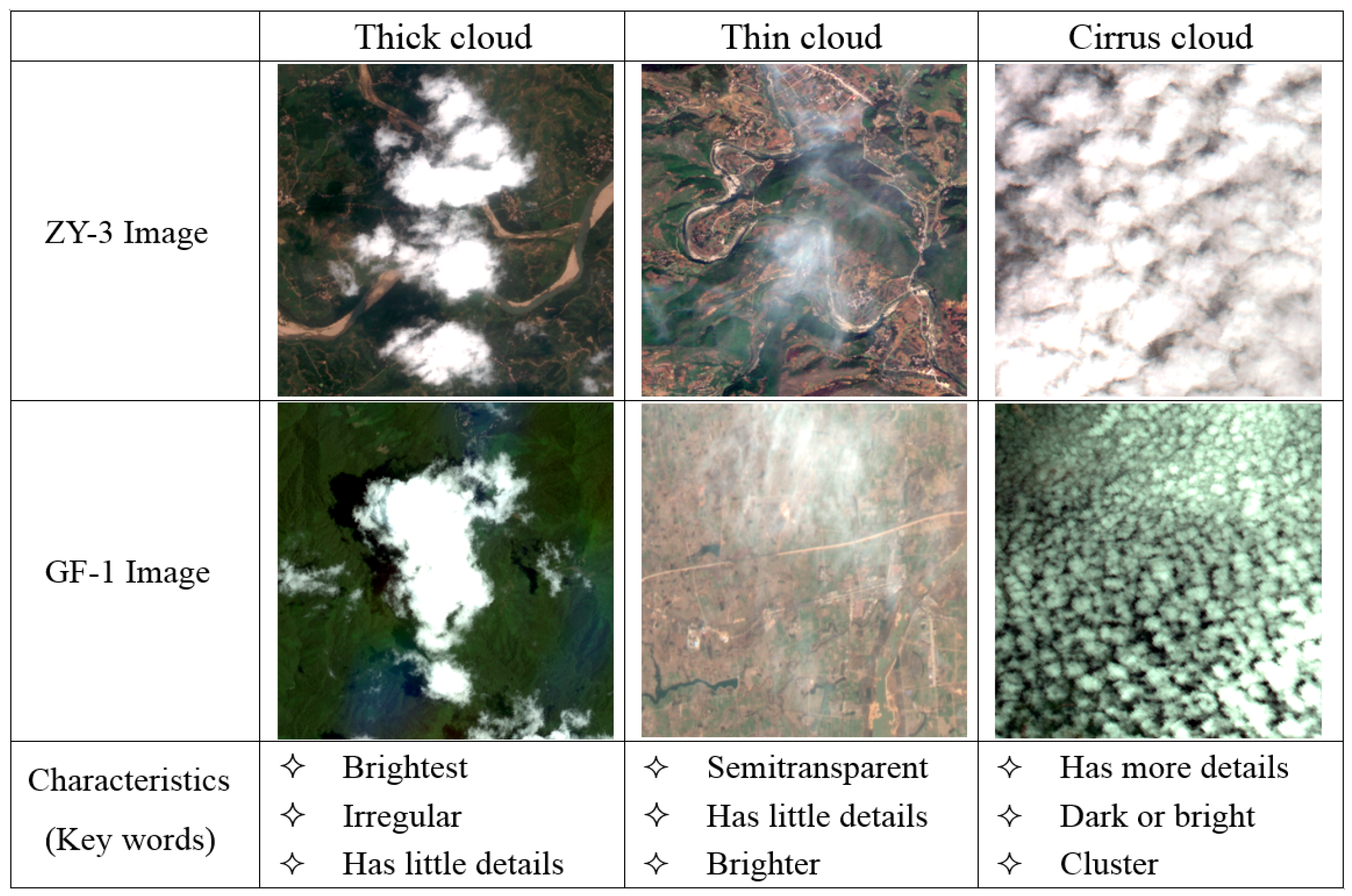
The basic features that are used for cloud detection in this paper are shown in
Figure 4. It can be seen that cloud regions usually share the following common properties:
Most cloud regions often have lower hues than non-cloud regions
Cloud regions generally have a higher intensity and NIR since the reflectivity of cloud regions is usually larger than that of non-cloud regions
Cloud regions generally have lower saturation since they are white in a RGB color model
The ground covered by a cloud veil usually has few details as the ground object features are all attenuated by clouds
Cloud regions always appear in terms of clustering
In addition, a remote sensing image can be converted from spatial domain to frequency domain by wavelet transform, which can decompose the image into low-frequency and high-frequency components. The objects that change dramatically in gray scale tend to be distributed in the high-frequency components, while those that change slowly, such as clouds, are distributed mainly in the low-frequency component.
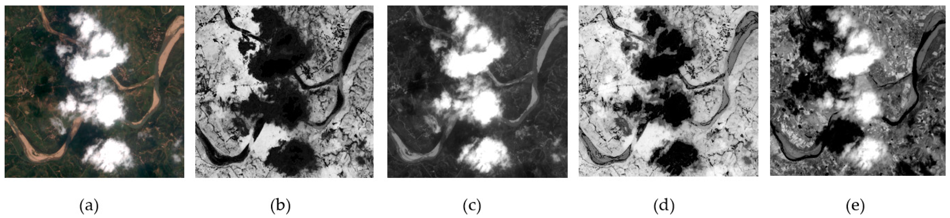
Based on the above features, more complicated features can be introduced as follows shown in
Figure 5.
(a) Spectral feature (SF): To highlight the difference between cloud regions and non-cloud regions, SF is extracted by constructing a significance map [
22]. This feature fully uses the properties that cloud regions in satellite images: higher intensity and lower hue, which can be written as:
where
and
refer to intensity and saturation bounded to (0, 1), respectively.
is an offset value, which provides an amplification of SF and ensure that the denominator is greater than 0. In this paper, we typically used
= 1.0. To obtain an intuitive visual description of SF, the value of SF is scaled to the range of (0, 255) (see
Figure 5b);
(b) Texture feature (TF): Ideal detail map can been extracted by multiple bilateral filtering [
22], which is effective but time-consuming. In the experiment, histogram equalization is presented in the intensity channel to highlight the implicit texture information; then, the texture feature can be extracted by applying bilateral filtering only once. As cloud regions in satellite images usually have fewer details compared to complex ground objects, this feature is an important clue to successful determination of non-cloud regions. The bilateral filtering is defined as:
where IE refers to the intensity enhanced by traditional histogram equalization.
denotes the filtered image from IE;
denotes the square window centered in
;
denotes the coordinates of the pixels within
;
denotes the calculated weight composed of space distance factor
and similarity factor
; and
and
are the standard deviations of the Gaussian function in the space domain and the color domain, respectively. If
is larger, the border pixels have a greater effect on the values of the center pixel. On the other hand, if
is larger, the pixels with a larger radiation difference with the center pixel are taken into the calculations. In the implementation process, we typically set the size of
to 2, and
to IEmax/10, which denotes the maximum value of intensity after histogram equalization. In the same way, the value of TF is scaled to the range of (0, 255) (see
Figure 5c);
(c) Frequency feature (FF): As clouds are always a low-frequency component in satellite images, the low-frequency information of the image is extracted by wavelet transform in intensity space [
8]. In this paper, we first used biorthogonal wavelet transform to convert an image from the spatial domain to the frequency domain (the number of layer was set to 2). Then the value of the pixels in the low-frequency components remained unchanged, and the pixels in the high-frequency component were set to 0. As can be seen in
Figure 5d, many of the non-cloud objects in the high-frequency component were filtered by this method.
(d) Line segment feature (LSF): Clouds are generally irregular in shape, and there are very few line segments in the cloud regions, especially in thick and thin cloud regions. However, most of the human-made objects have a flat surface, so the line segments can be used to distinguish clouds from human-made objects. In this paper, the line segments are identified by line segment detector (LSD) algorithm [
28] (see
Figure 5e).
3.2.2. Background Superpixels (BS) Extraction
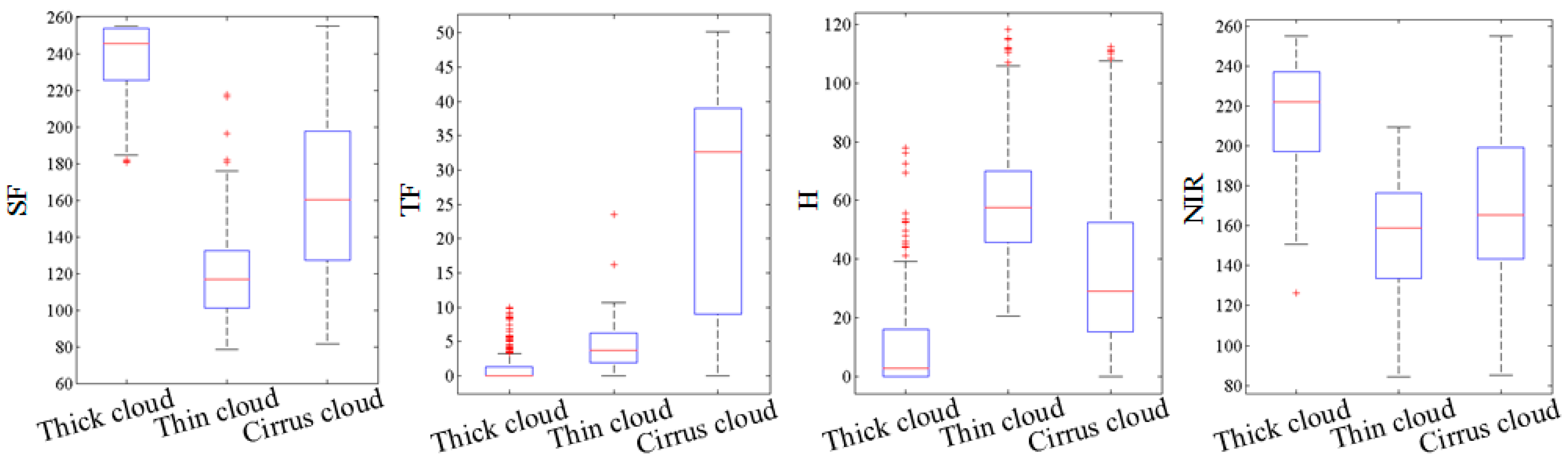
The basic premise of cloud detection is that cloud regions usually have higher SF, H, and NIR values, but the response in the space of TF and LSF is less than in the non-cloud regions and is always present in the low-frequency component. In fact, the greatest challenges for cloud detection are snow, buildings, sand, and bare land because they have high spectral reflectance in the visible bands. To improve the robustness and efficiency of cloud detection, some obvious background objects, such as water area, shadow, forest, and grass, can be extracted easily using the features introduced in the above section. To identify the distributions law of the features of true cloud superpixels, 500 superpixels for each type of cloud were collected. The average SF, TF, H, and NIR for each superpixel was counted and shown in
Figure 6. In order to keep the same intuitive visual description with SF and TF, the value of H and NIR were scaled to (0, 255). The specific dataset collection process of the proposed method therefore is as follows: (1) cloud images covering every season are selected; (2) all of the images are segmented into superpixels; (3) the average value of each feature is calculated for each superpixel; and (4) 500 superpixels are selected for each type of cloud, and the statistics for their feature values are obtained artificially.
Based on the SF information, the background superpixels from the input image can be identified coarsely by using a global thresholding method, such as Otsu’s method [
29]. However, due to the threshold shifting problem of Otsu’s method, some cloud superpixels may be missed when a prohibitively high Otsu’s threshold
is selected. Conversely, an excessive number of non-cloud superpixels may be mistaken for cloud superpixels when a prohibitively low Otsu’s threshold
is selected [
22]. To ensure detection accuracy, this paper proposes an optimal threshold T setting by adding an appropriate constraint to
. Based on the above observation, over 99.3% of the cloud superpixels were found to have a SF not less than 80. Thus, 80 was set as the lowest bound, which means that if Otsu’s threshold is lower than 80, the proposed method takes the optimal threshold of 80. Otherwise, Otsu’s threshold is selected. In the same way, the upper bound was set at 130, which was founded to be suitable for protecting the cloud superpixels. The formula for obtaining optimal threshold T is shown below:
In
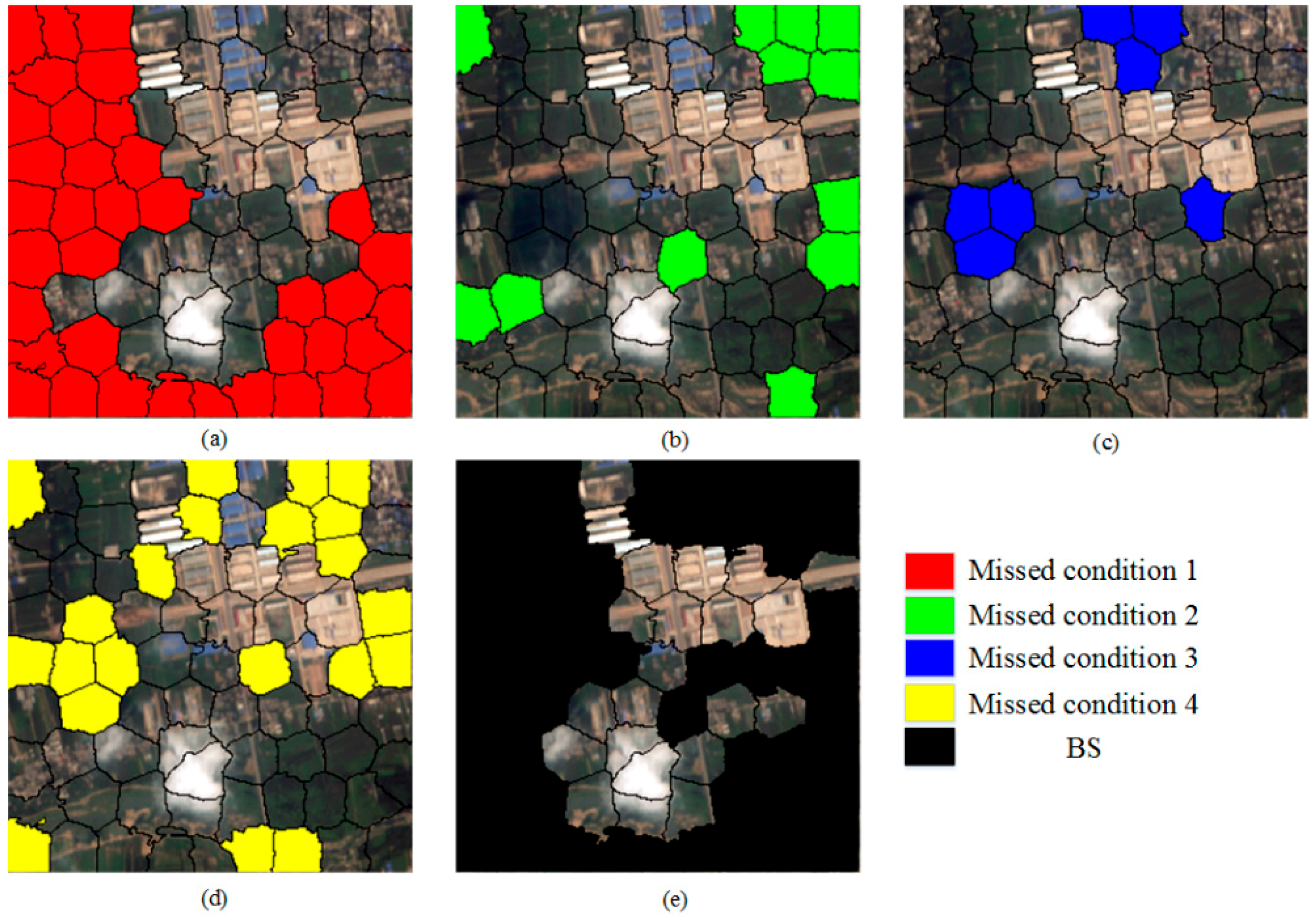
Figure 6, it can be see that although the feature values of TF, H, and NIR for different cloud types were different, but most all of these cloud superpixels had a TF of less than 50, their H was less than 120, and the NIR was more than 85. Therefore, it was concluded that true cloud superpixels must meet the following conditions:
Condition 1: The feature value of SF is larger than optimal threshold T;
Condition 2: The feature value of TF is less than 50;
Condition 3: The feature value of H is less than 120;
Condition 4: The feature value of NIR is not less than 85.
Superpixels are defined as BS if none of these four conditions is satisfied. One example of BS extraction based on four conditions is shown in
Figure 7.
3.2.3. Cloud Mask Extraction
SF, TF, and FF usually distinguishing different targets well. However, the same target may present different features, and different targets may present similar features in complex satellite images. Thus, problems of ambiguity and similarity between the feature vectors and the target semantics may appear and obtaining the true semantics of the target for machine learning algorithms in the case of inadequate training samples is a difficult process. To solve these problems, bag-of-words (BOW), latent semantic analysis (LSA), PLSA, and other were introduced in computer vision. T. Hofmann, et al. (2001) experimentally verified that PLSA is more principled than BOW and LSA in extracting latent features semantics, since PLSA possess a sound statistical foundation and utilizes the (annealed) likelihood function as an optimization criterion [
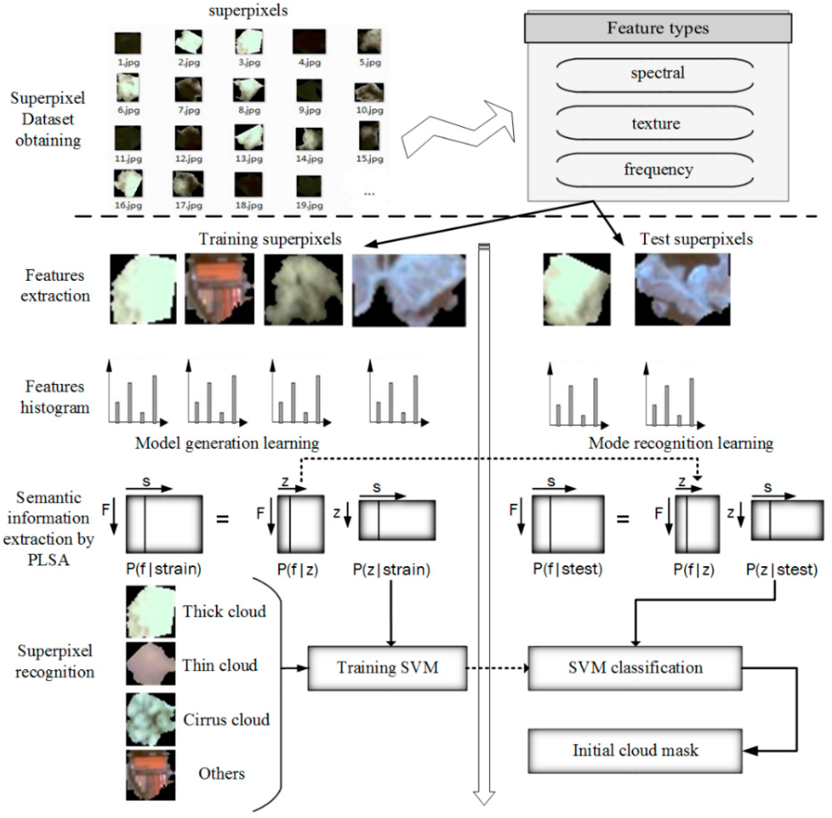
30]. In this paper, the PLSA model therefore was applied to training typical images, and the targets then were recognized based on the PLSA distribution. The workflow of the cloud mask extraction process is shown in
Figure 8.
The detailed recognition steps are as follows:
(a) Superpixel dataset obtaining.
Remote sensing images are segmented into superpixels, and the cloud and non-cloud superpixels are selected as the training dataset. In theory, the more training samples there are, the better the results are; and the number of negative samples should be twice the number of positive samples.
(b) Features extraction.
Feature selection is a very important step in superpixels recognition. In this paper,
, was extracted for each superpixel (both the training superpixels and test superpixels); and n denotes the number of pixels in the superpixel and
,
,
denote the SF, TF, FF values of pixel n, respectively. As can be seen in
Figure 5, the SF and FF values of a cloud pixel were very large, but the TF value was small. To promote the same trend in the experiments in this paper,
was utilized.
(c) Features histogram.
Since the features of each superpixel are extracted, an appropriate vector to describe every superpixel is need. In this paper, the features histogram
was counted for superpixels
as the feature descriptor as shown in
Figure 9. Where M is the maximum feature value in the imagery, since SF, TF, and FF were scaled to the range of (0, 255), M was set at 255 in this experiment.
denotes the percentage of value M in STF, and O denotes the number of superpixels. Thereafter, the matrix of characteristic frequency
was obtained, where
denotes the frequency of feature
appears in superpixel
. In addition, each
corresponds to a set of underlying themes
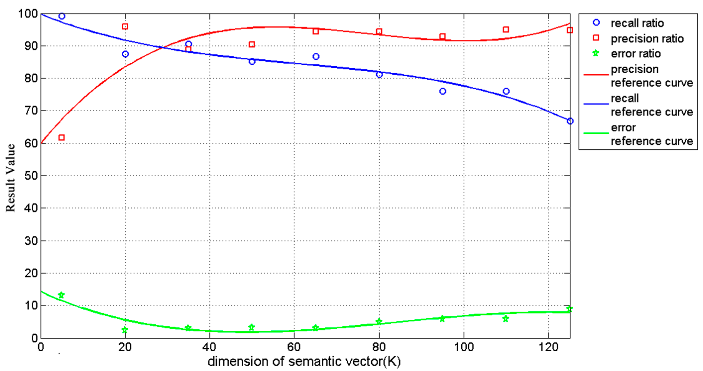
. K indicates the number of themes, which was set at 20 in this paper. The effect of parameter K for cloud detection is analyzed in
Section 4.2.
(d) Semantic information extraction by PLSA.
This step includes model generation learning and model recognition learning.
(1) Model generation learning. To obtain the distribution pattern
of the features of the training superpixels when the latent semantic appears, the approximate solution of the PLSA model was calculated by Expectation-Maximization (EM) algorithm iteratively [
30]. The E-step and the M-step are included in this process and are described below:
E-step, the posteriori probability of the underlying theme information for each superpixel
can be computed by
where
denotes the probability of the underlying theme
that appears in
, and denotes the probability of superpixel
appearing in underlying theme
. In this paper;
and
were initialized by using pseudorandom number generators.
M-step, re-estimation of
, and
are based on the posteriori probability by
where
denotes probability of the feature
of superpixel
appearing in the underlying theme
. The EM algorithm is used iteratively, until
(see Formula (16)) becomes stable, then the distribution pattern
of the features of training superpixels are obtained when the latent semantic appears.
(2) Model recognition learning. Using the distribution pattern obtained, for any test superpixel , a K dimension semantic vector can be constructed to describe it. First, histogram feature vector of the superpixel is extracted. Then, and are taken into the EM algorithm as described above. Finally, semantic vector is calculated, which has the same dimension with Z. Each value in the semantic vector represents the probability of this superpixel belonging to a corresponding theme, and the sum of them should be 1.0. If two superpixels are the same class, such as thick cloud, their semantic vectors will be similar; but the difference between the semantic vectors of a thick cloud superpixel and a vegetation superpixel will be very large.
(e) Superpixel recognition.
K dimensions semantic vector
describes the superpixel, which then can be recognized by the machine-learning algorithm. A series of state-of-the-art algorithms recently were developed for remote-sensing image classification, such as SVM, Extreme Learning Machine (ELM), Decision Tree, Random Forest (RF) and Tree Bagger (TB). Huang, et al. (2015) experimentally verified that SVM outperformed other machine-learning methods in target extraction from remote sensing images. In addition, RBF-SVM demonstrated the best stability for non-linear classification [
31]. In this paper, the result is a non-linear classification model that can be used to classify new test superpixel. Thus, the Radial Basis Function (RBF) kernel was selected as the kernel function of SVM and a five-fold cross-validation was conducted to determine the optimal parameters. The steps of recognition by SVM are as follows:
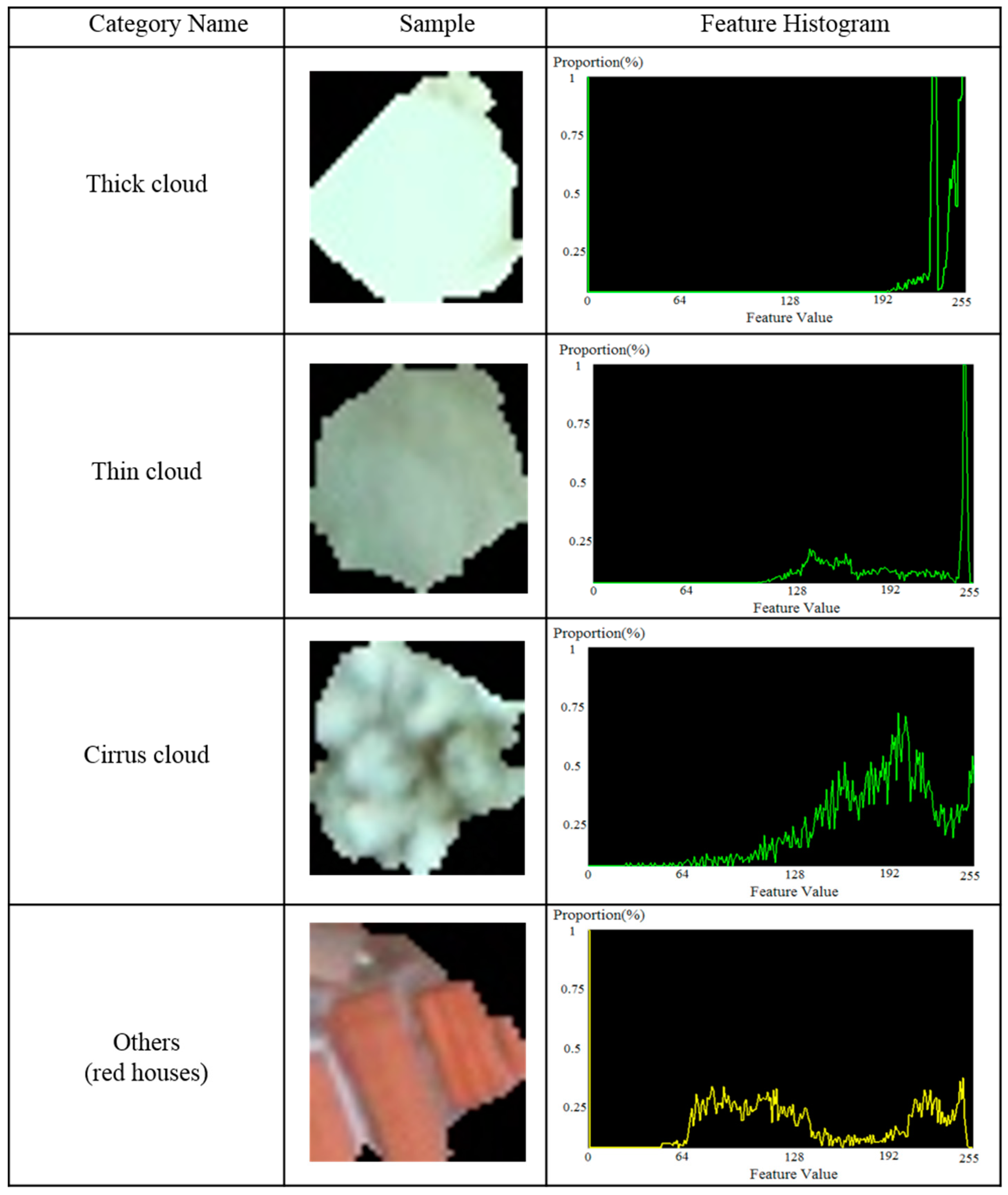
(1) Cloud superpixels are divided into four categories, thin cloud, thick cloud, cirrus cloud, and others. A set of training samples for each category are selected.
(2) The semantic vector of each training sample of each category is extracted by the method described as above (see model recognition learning).
(3) A classification model is obtained using the training samples by SVM.
(4) For any test sample, the semantic vector is extracted, then the sample will be recognized by using the classification model.
A series of GF-1 images were selected as the training examples. All of the images were segmented into superpixels, and a training set was obtained by visual interpretation. In the experiment, there were four categories: thick cloud, thin cloud, cirrus cloud, and others; and 600 positive samples (include 200 thick cloud superpixels, 200 thin cloud superpixels, and 200 cirrus cloud superpixels) and 1000 negative samples (forest, cities and towns, river, barren land, etc.) were collected in advance.
Figure 9 shows the four categories and the corresponding features histogram STFH discussed above.
The semantic vectors
of the superpixels were counted by PLSA, and the classification model was obtained by RBF-SVM, after which the test superpixels were recognized as one of the categories. In fact, the experiments determined that cirrus clouds were more difficult to distinguish from background superpixels than thick clouds and thin clouds. In
Figure 6, it also can be seen that the feature values of SF and TF for cirrus cloud superpixels highly overlapped. Although the proposed method improved the accuracy of cirrus cloud superpixels recognition, 100% accuracy cannot be ensured. Thus, if superpixels were recognized as cirrus clouds, they were designated as possible foreground superpixels (PFS); if superpixels were recognized as thick or thin clouds, they were designated as foreground superpixels (FS); and if superpixels were recognized as others, they were designated as possible background superpixels (PBS).
In the experiments, large white buildings and snow were difficult to distinguish from thick clouds. According to the previous description (see
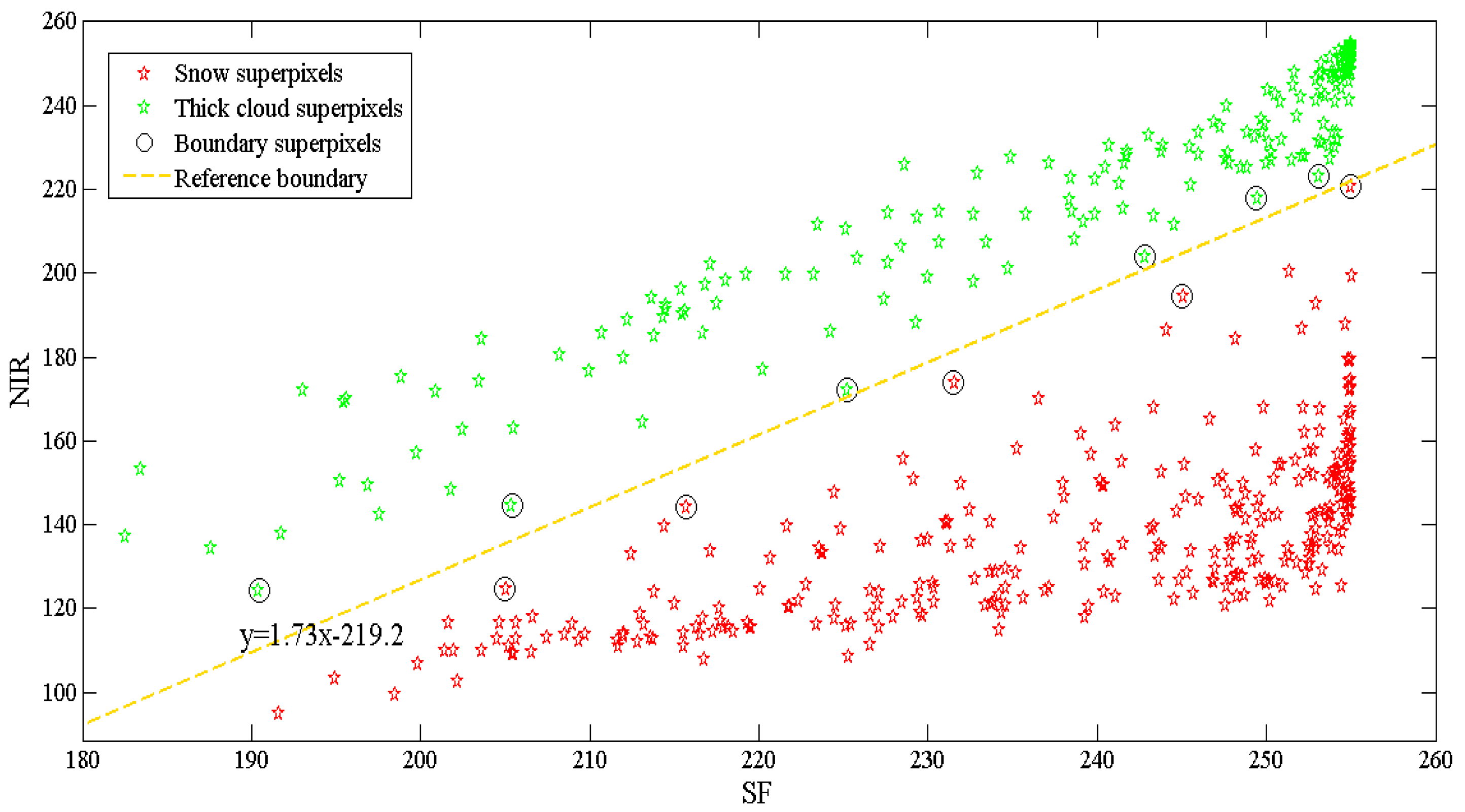
Section 3.2.1), LSF is helpful in distinguishing thick clouds from human-made objects. Thus, in order to refine the cloud mask, if the line segments can be extracted in the FS, then they can be turned as BS forcibly. In addition, snow superpixels were found to always have a lower NIR than thick cloud superpixels. This phenomenon can be clearly observed in
Figure 10, where 500 selected thick cloud superpixels and snow superpixels are shown, as well as the relationship between SF and NIR. A clearly boundary was visible between snow and thick clouds. The boundary superpixels were selected and fitted to the reference boundary by the Least Squares algorithm. Then,
was computed; if ST was smaller than 0, FS was turned to PBS forcibly.
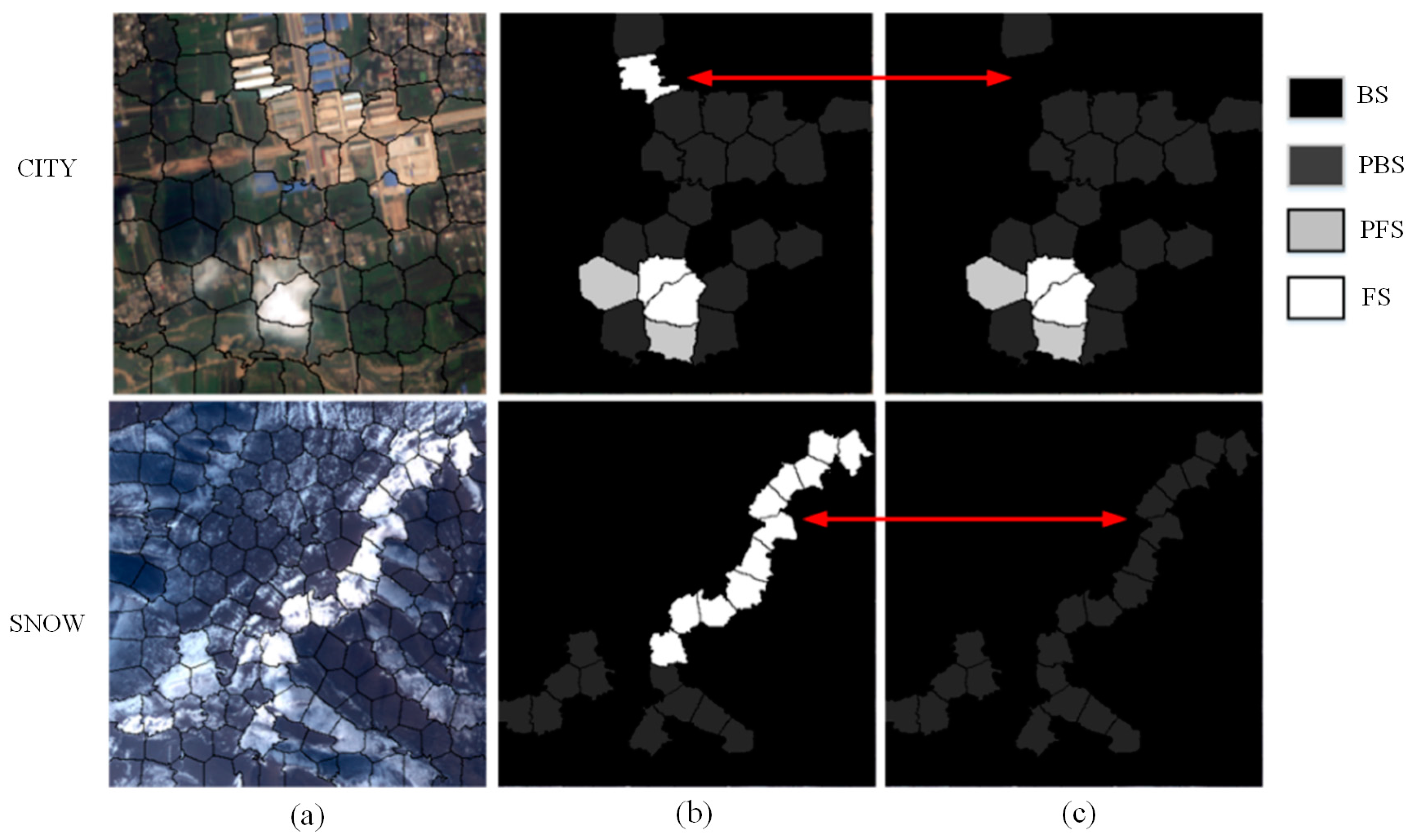
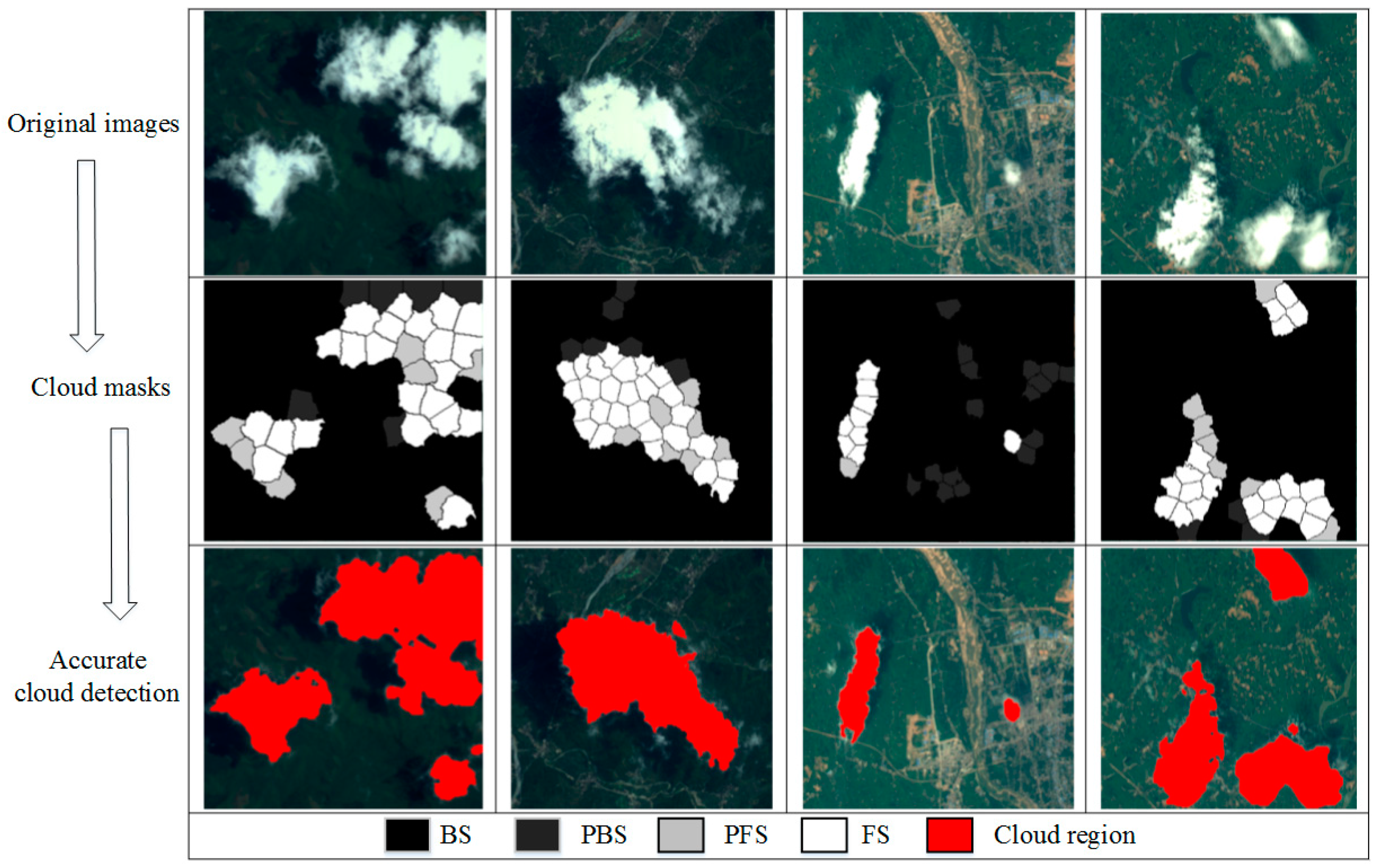
According to the above processes, a good cloud mask can be obtained at the superpixel level. In this study, two typical scenes, city and snow, were selected as the test examples. The results of the cloud mask extraction are shown in
Figure 11. It can be seen that the proposed method can generate satisfactory results for complex satellite images. Superpixels with large areas of clouds were accurately recognized as the interest targets, and the superpixels with small or no content of clouds were eliminated effectively. Furthermore, these processes were robust enough to exclude some problems that are difficult to solve with traditional spectral-based methods. As can be seen in
Figure 11, the superpixels of white buildings, bright roads, frost, snow, and barren lands were effectively eliminated and semitransparent cloud superpixels were accurately extracted.


