1. Introduction
High-resolution digital terrain models (DTMs) are critical for flood simulation, landslide monitoring, road design, land-cover classification, and forest management [
1]. Light detection and ranging (LiDAR) technology, which is an efficient way to collect three-dimensional point clouds over a large area, has been widely used to produce DTMs. To generate DTMs, ground and non-ground measurements have to be separated from the LiDAR point clouds, which is a filtering process. Consequently, various types of filtering algorithms have been proposed to automatically extract ground points from LiDAR point clouds. However, develo** an automatic and easy-to-use filtering algorithm that is universally applicable for various landscapes is still a challenge.
Many ground filtering algorithms have been proposed during previous decades, and these filtering methods can be mainly categorized as slope-based methods, mathematical morphology-based methods, and surface-based methods. The common assumption of slope-based algorithms is that the change in the slope of terrain is usually gradual in a neighborhood, while the change in slope between buildings or trees and the ground is very large. Based on this assumption, Vosselman [
2] developed a slope-based filtering algorithm by comparing slopes between a LiDAR point and its neighbors. To improve the calculation efficiency, Shan and Aparajithan [
3] calculated the slopes between neighbor points along a scan line in a specified direction, which was extended to multidirectional scan lines by Meng
et al. [
4]. Acquiring an optimal slope threshold that can be applied to terrain with different topographic features is difficult with these methods. To overcome this limitation, various automatic threshold definitions have been studied, e.g., adaptive filters [
5,
6] and dual-direction filters [
7]. Nonetheless, their results suggested that slope-based algorithms were not guaranteed to function well in complex terrain, as the filtering accuracy decreased with increasingly steeper slopes [
8].
Another type of filtering method uses mathematical morphology to remove non-ground LiDAR points. Selecting an optimal window size is critical for these filtering methods [
9]. A small window size can efficiently filter out small objects but preserve larger buildings in ground points. On the other hand, a large window size tends to smooth terrain details such as mountain peaks, ridges and cliffs. To solve this problem, Zhang
et al. [
10] developed a progressive morphological filter to remove non-ground measurements by comparing the elevation differences of original and morphologically opened surfaces with increasing window sizes. However, poor ground extraction results may occur because the terrain slope is assumed to be a constant value in the whole processing area. To overcome this constant slope constraint, Chen
et al. [
11] extended this algorithm by defining a set of tunable parameters to describe the local terrain topography. Other improved algorithms that are based on mathematical morphology can be found in [
12,
13,
14,
15]. The advantage of mathematical morphology-based methods is that they are conceptually simple and can be easily implemented. The accuracy of morphological based approach is also relatively good. However, additional priori knowledge of the study area is usually required to define a suitable window size because local operators are used [
16].
Previous algorithms separated ground and non-ground measurements by removing non-ground points from LiDAR datasets. In contrast to these algorithms, surface-based methods gradually approximate the ground surface by iteratively selecting ground measurements from the original dataset, and the core of this type of filtering method is to create a surface that approximates the bare earth. Axelsson [
17] proposed an adaptive triangulated irregular network (TIN) filtering algorithm that gradually densified a sparse TIN that was generated from the selected seed points. In this algorithm, two important threshold parameters need to be carefully set: one is the distance of a candidate point to the TIN facet, and the other is the angle between the TIN facet and the line that connects the candidate point with the facet’s closest vertex. These parameters are constant values for the entire study area in the adaptive TIN filter, which makes it difficult to detect ground points around break lines and steep terrain. Recently, Zhang and Lin [
18] improved this algorithm by embedding smoothness-constrained segmentation to handle surfaces with discontinuities. Another typical surface-based filtering algorithm was developed by Kraus and Pfeifer [
19], who used a weighted linear least-squares interpolation to identify ground points from LiDAR data. This algorithm was first used to remove tree measurements and generate DTMs in forest areas and was subsequently extended to process LiDAR points in urban areas by incorporating a hierarchical approach [
20]. By using this filtering algorithm, ground measurements can be successfully detected on flat terrain, but the filtering results are less reliable on terrain with steep slopes and large variability. To cope with this problem, multi-resolution hierarchical filtering methods have been proposed to identify ground LiDAR points based on point residuals from a thin plate spline-interpolated surface [
16,
21,
22]. Recently, Hui
et al. [
23] proposed an improved filtering algorithm which combines the traditional morphological filtering algorithm and multi-level interpolation filtering algorithm. It can achieve promising results in both of urban areas and rural areas.
Another special surface-based filtering algorithm was proposed by Elmqvist [
24], who employed active shape models to approximate the ground surface. In this algorithm, an energy function is designed as a weighted combination of internal forces from the shape of the contour and external forces from the LiDAR point clouds. Minimizing this energy function determines the ground surface, which behaves like a membrane that sticks to the lowest points. This algorithm is a new idea to model ground surface from LiDAR data, but the optimization only achieve an global optimum solution, which does not guarantee to get all the local optimums. Thus, some local details may be ignored. Meanwhile, this algorithm performs relatively poorly in complex areas as reported in [
25]. They may also fail to effectively model terrain with steep slopes and large variability because they are based on the assumption that the terrain is a smooth surface. Furthermore, another challenge of these methods is how to increase the efficiency when the accuracy is fixed [
18].
The use of the aforementioned filtering algorithms has proven to be successful, but the performance of these algorithms changes according to the topographic features of the area, and the filtering results are usually unreliable in complex cityscapes and very steep areas. In addition, the implementation of these filtering methods requires a number of suitable parameters to achieve satisfactory results, which are difficult to determine because the optimal filter parameters vary from landscape to landscape, so these filtering methods are not easy to use by users without much experience. To cope with these problems, this paper proposes a novel filtering algorithm which is capable of approximating the ground surface with a few parameters. Different from other algorithms, the proposed method filters the ground points by simulating a physical process that an virtual cloth drops down to an inverted (upside-down) point cloud. Compared to existing filtering algorithms, the proposed filtering method has some advantages: (1) few parameters are used in the proposed algorithm, and these parameters are easy to understand and set; (2) the proposed algorithm can be applied to various landscapes without determining elaborate filtering parameters; and (3) this method works on raw LiDAR data.
The remainder of this paper is organized as follows. A new ground filtering algorithm is proposed in
Section 2.
Section 3 presents the experimental results, and the proposed algorithm is discussed in
Section 4. Finally,
Section 5 concludes this paper.
2. Method
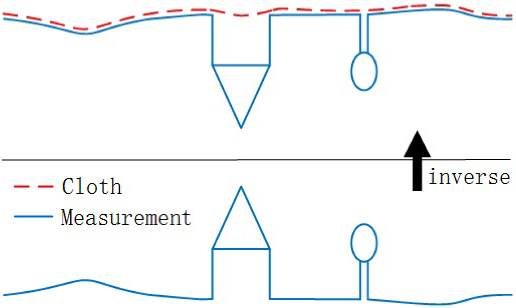
Our method is based on the simulation of a simple physical process. Imagine a piece of cloth is placed above a terrain, and then this cloth drops because of gravity. Assuming that the cloth is soft enough to stick to the surface, the final shape of the cloth is the DSM (digital surface model). However, if the terrain is firstly turned upside down and the cloth is defined with rigidness, then the final shape of the cloth is the DTM. To simulate this physical process, we employ a technique that is called cloth simulation [
26]. Based on this technique, we developed our cloth simulation filtering (CSF) algorithm to extract ground points from LiDAR points. The overview of the proposed algorithm is illustrated in
Figure 1. First, the original point cloud is turned upside down, and then a cloth drops to the inverted surface from above. By analyzing the interactions between the nodes of the cloth and the corresponding LiDAR points, the final shape of the cloth can be determined and used as a base to classify the original points into ground and non-ground parts.
2.1. Fundamental of the Cloth Simulation
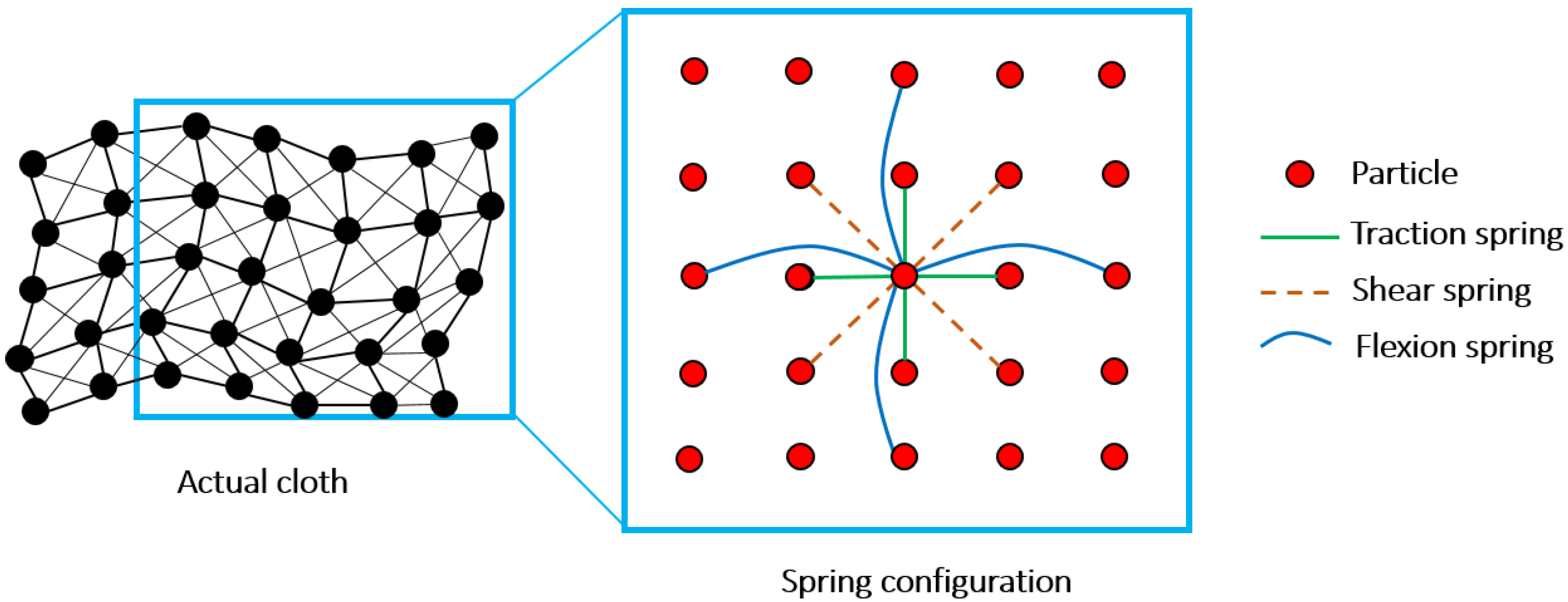
Cloth simulation is a term of 3D computer graphics. It is also called cloth modeling, which is used for simulating cloth within a computer program. During cloth simulation, the cloth can be modeled as a grid that consists of particles with mass and interconnections, called a Mass-Spring Model [
27].
Figure 2 shows the structure of the grid model. A particle on the node of the grid has no size but is assigned with a constant mass. The positions of the particles in three-dimensional space determine the position and shape of the cloth. In this model, the interconnection between particles is modeled as a “virtual spring”, which connects two particles and obeys Hooke’s law. To fully describe the characteristics of the cloth, three types of springs have been defined: shear spring, traction spring and flexion spring. A detailed description about the functions of these different springs can be found in [
27].
To simulate the shape of the cloth at a specific time, the positions of all of the particles in the 3D space are computed. The position and velocity of a particle are determined by the forces that act upon it. According to Newton’s second law, the relationship between position and forces is determined by Equation (
1):
where
X means the position of a particle at time
t;
stands for the external force, which consists of gravity and collision forces that are produced by obstacles when a particle meets some objects in the direction of its movement; and
stands for the internal forces (produced by interconnections) of a particle at position
X and time
t. Because both the internal and external forces vary with time
t, Equation (
1) is usually solved by a numerical integration (e.g., Euler method) in the conventional implementation of cloth simulation.
2.2. Modification of the Cloth Simulation
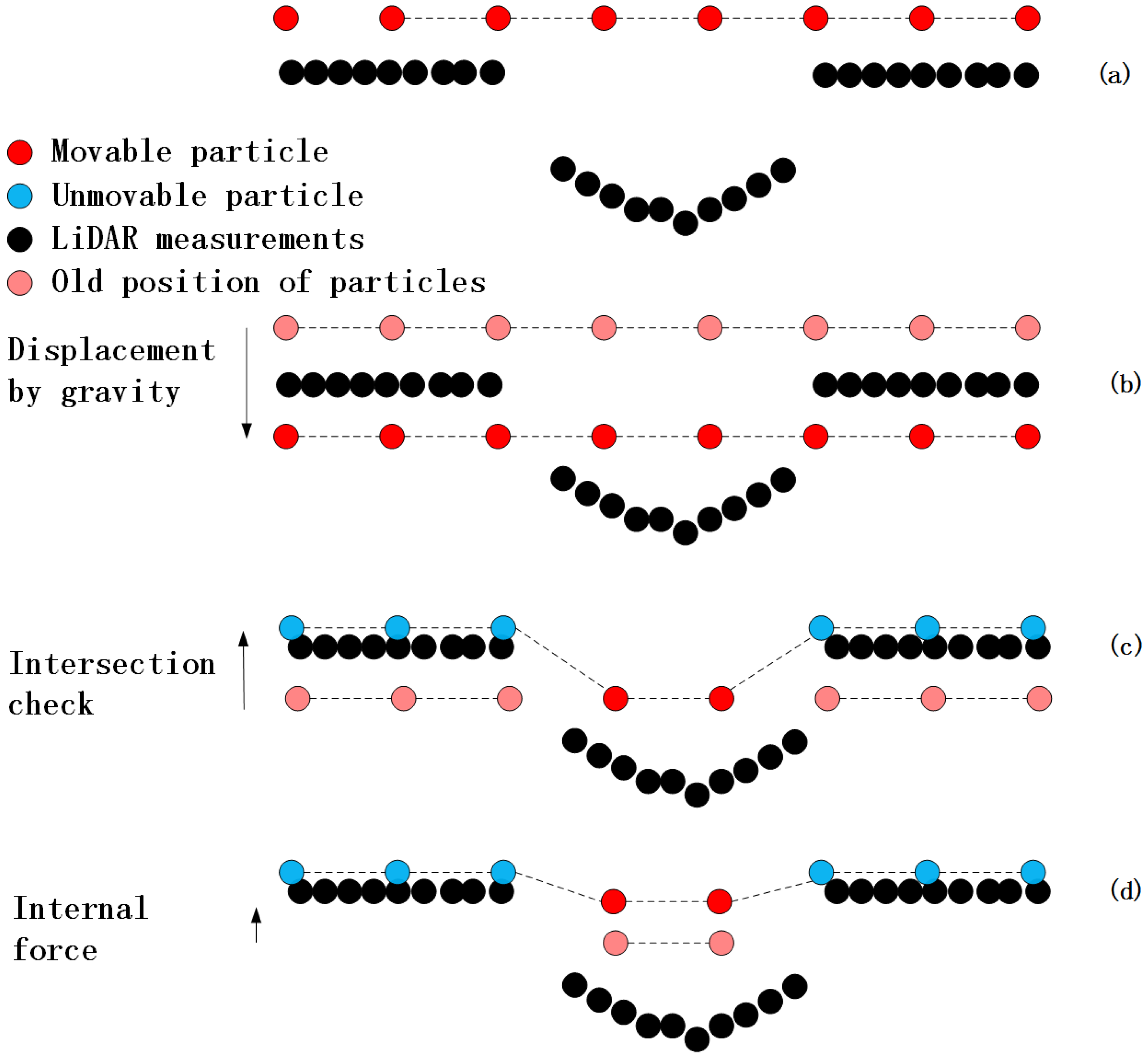
When applying the cloth simulation to LiDAR point filtering, a number of modifications have been made to make this algorithm adaptable to point cloud filtering. First, the movement of a particle is constrained to be in vertical direction, so the collision detection can be implemented by comparing the height values of the particle and the terrain (e.g., when the position of a particle is below or equal to the terrain, the particle intersects with the terrain). Second, when a particle reaches the “right position”,
i.e., the ground, this particle is set as unmovable. Third, the forces are divided into two discrete steps to achieve simplicity and relatively high performance. Usually, the position of a particle is determined by the net force of the external and internal forces. In this modified cloth simulation, we first compute the displacement of a particle from gravity (the particle is set as unmovable when it reaches the ground, so the collision force can be omitted) and then modify the position of this particle according to the internal forces. This process is illustrated in
Figure 3.
2.3. Implementation of CSF
As described above, the forces that act on a particle are considered as two discrete steps. This modification was inspired by [
28]. First, we calculate the displacement of each particle only from gravity,
i.e., solve Equation (
1) with internal forces equal to zero. Then, the explicit integration form of this equation is
where
m is the mass of the particle (usually,
m is set to 1) and
is the time step. This equation is very simple to solve. Given the time step and initial position, the current position can be calculated directly because
G is a constant.
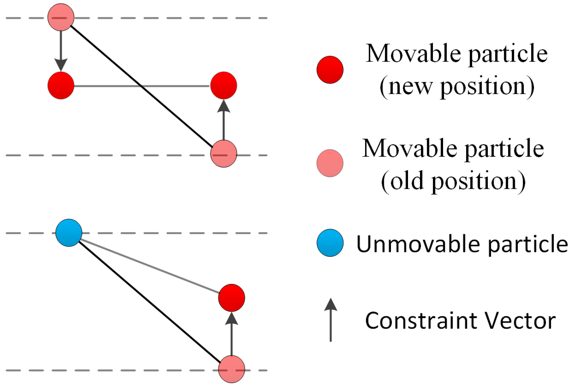
To constrain the displacement of particles in the void areas of the inverted surface, we consider the internal forces at the second step after the particles have been moved by gravity. Because of internal forces, particles will try to stay in the grid and return to the initial position. Instead of considering neighbors of each particle one by one, we simply traverse all the springs. For each spring, we compare the height difference between the two particles which form this spring. Thus, the 2-dimensional (2-D) problem are abstracted as a one-dimensional (1-D) problem, which is illustrated in
Figure 4.
As we have restricted the movement directions of the particles, two particles with different height values will try to move to the same horizon plane (cloth grid is horizontally placed at the beginning). If both connected particles are movable, we move them by the same amount in the opposite direction. If one of them is unmovable, then the other will be moved. Otherwise, if these two particles have the same height value, neither of them will be moved. Thus, the displacement (vector) of each particle can be calculated by the following equation:
where
represents the displacement vector of a particle;
b equals to 1 when the particle is movable, otherwise it equals to 0.
is the position of current particle that is ready to be moved.
is the position neighboring particle that connects with
; and
is a normalized vector that points to vertical direction,
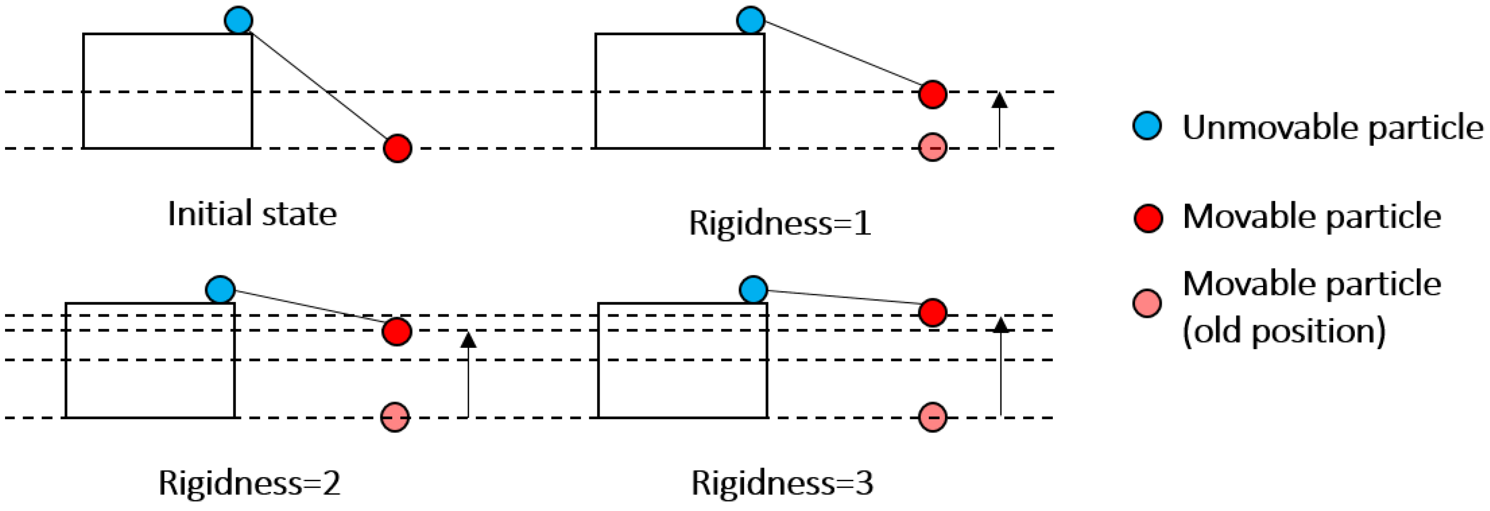
. This movement process can be repeated; we set a parameter rigidness (
) to represent the repeated times. This parameterization process is shown in
Figure 5. If
is set to 1, the movable particle is just moved only once, and the displacement is half of the vertical distance (VD) between the two particles. If the
is set to 2, the movable particle will be moved twice, the total displacement is 3/4VD. Finally, if
is set to 3, the movable particle will be moved three times and the total displacement is 7/8VD. The value of 3 is enough to produce a very hard cloth. Thus, we constrain the rigidness to values of 1, 2 and 3. The larger the rigidness is, the more rigidly the cloth will behave.
The main implementation procedures of CSF are described as follows. First, we project the cloth particles and LiDAR points into the same horizontal plane and then find a nearest LiDAR point (named corresponding point, CP) for each cloth particle in this 2D plane. An intersection height value (IHV) is defined to record the height value (before projection) of CP. This value represents the lowest position that a particle can reach (i.e., if the particle reaches the lowest position that is defined by this value, it cannot move forward anymore). During each iteration, we compare the current height value (CHV) of a particle with IHV; if CHV is equal or lower than IHV, we move the particle back to the position of IHV and make the particle unmovable.
An approximation of the real terrain is obtained after the simulation, and then the distances between the original LiDAR points and simulated particles are calculated by using a cloud-to-cloud distance computation algorithm [
29]. LiDAR points with distances that are less than a threshold
are classified as BE (bare earth), while the remaining points are OBJ (objects).
The procedure of the proposed filtering algorithm is presented as follows:
Automatic or manual outliers handling using some third party software (such as cloudcompare).
Inverting the original LiDAR point cloud.
Initiating cloth grid. Determining number of particles according to the user defined grid resolution (GR). The initial position of cloth is usually set above the highest point.
Projecting all the LiDAR points and grid particles to a horizontal plane and finding the CP for each grid particle in this plane. Then recording the IHV.
For each grid particle, calculating the position affected by gravity if this particle is movable, and comparing the height of this cloth particle with IHV. If the height of particle is equal to or less than IHV, then this particle is placed at the height of IHV and is set as “unmovable”.
For each grid particle, calculating the displacement of each particle affected by internal forces.
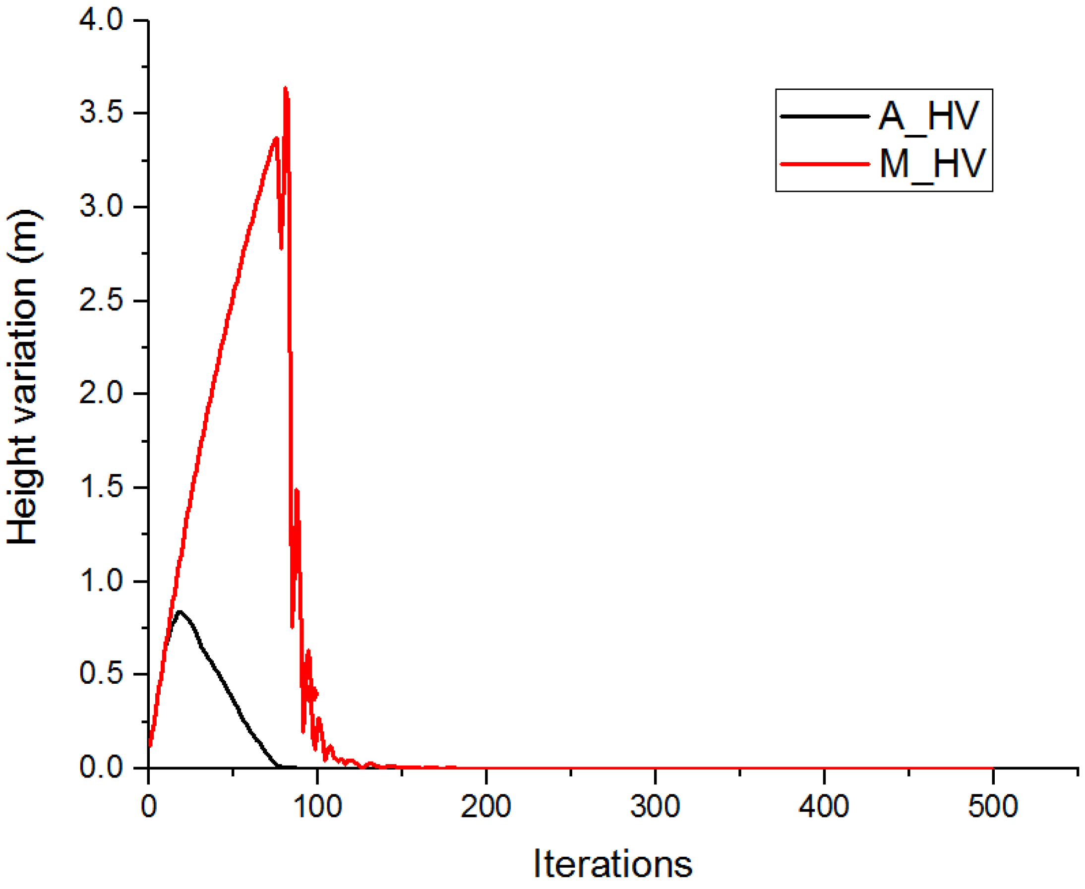
Repeating (5)–(6). The simulation process will terminate when the maximum height variation (M_HV) of all particles is small enough or when it exceeds the maximum iteration number which is specified by the user.
Computing the cloud to cloud distance between the grid particles and LiDAR point cloud.
Differentiating ground from non-ground points. For each LiDAR points, if the distance to the simulated particles is smaller than , this point is classified as BE, otherwise it is classified as OBJ.
2.4. Post-Processing
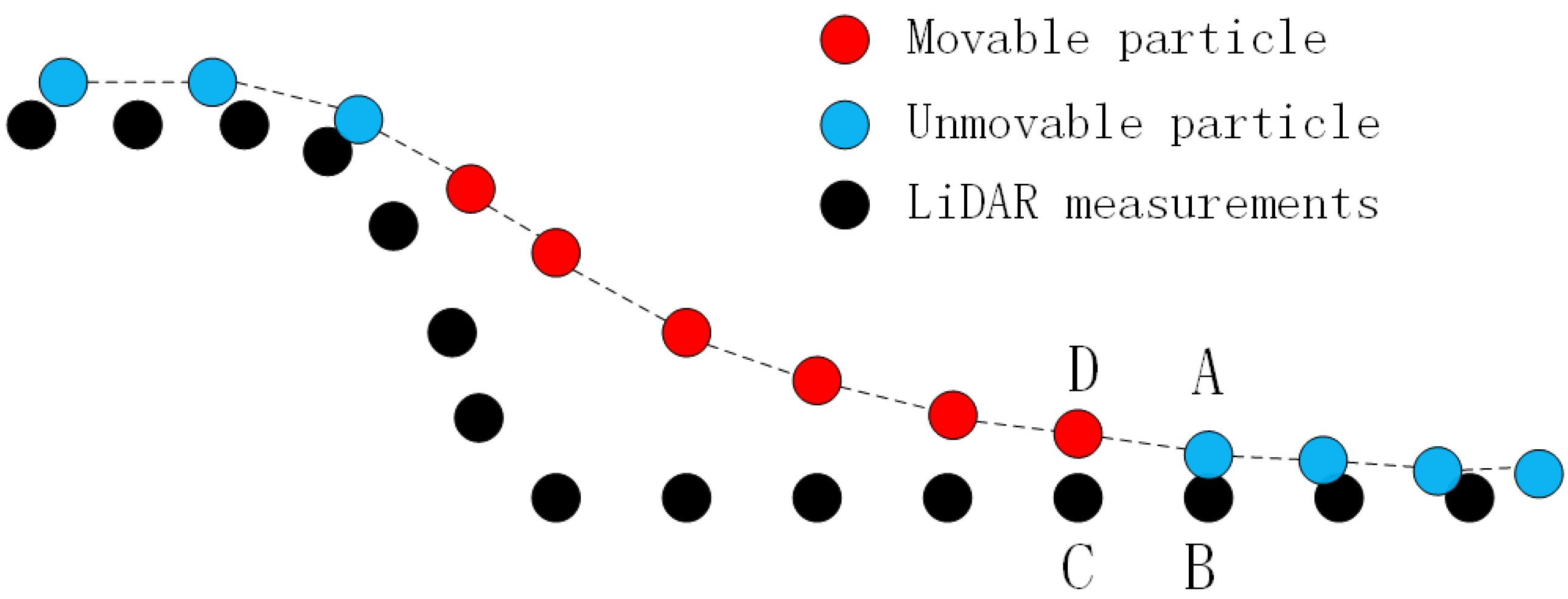
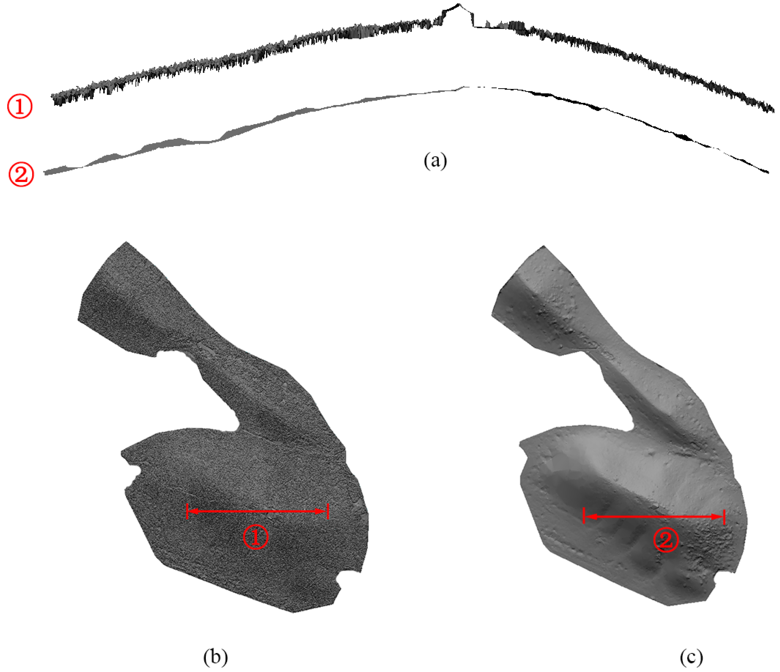
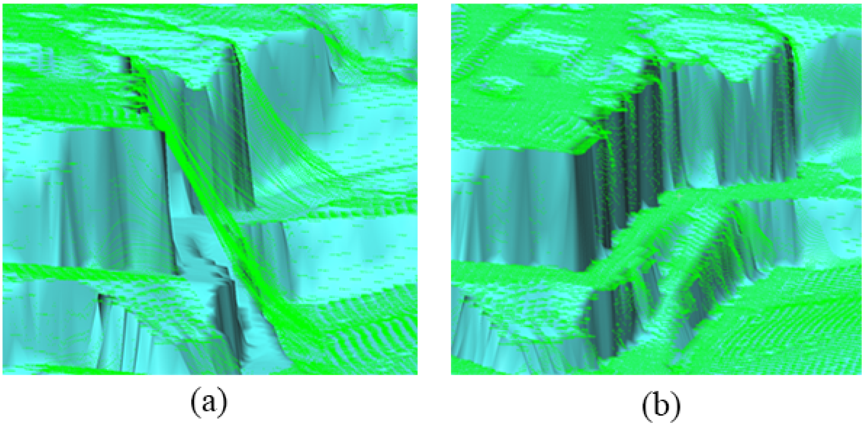
For steep slopes, this algorithm may yield relatively large errors because the simulated cloth is above the steep slopes and does not fit with the ground measurements very well due to the internal constraints among particles, which is illustrated in
Figure 6. Some ground measurements around steep slopes are mistakenly classified as OBJ. This problem can be solved by a post-processing method that smoothes the margins of steep slopes. This post-processing method finds an unmovable particle in the four adjacent neighborhoods of each movable particle and compares the height values of CPs. If the height difference is within a threshold (
), the movable particle is moved to the ground and set as unmovable. For example, for point D in
Figure 6, we find that point A is the unmovable particle from the four adjacent neighbors of D. Then, we compare the height values between C and B (the CPs for D and A, respectively). If the height difference is less than
, then this candidate point D is moved to C and is set as unmovable. We repeat this procedure until all the movable particles are properly handled (either set as unmovable or kept movable).
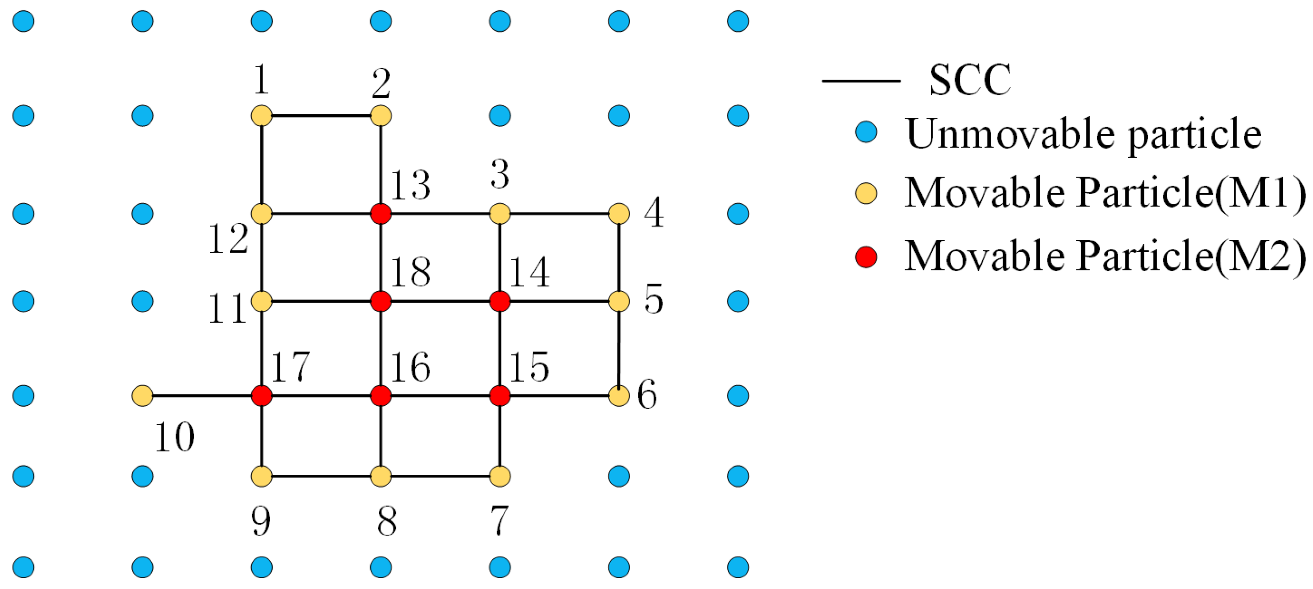
To implement post-processing, all the movable particles should be traversed, if we scan the cloth grid row by row, the results may be affected by this particular scan direction. Thus, we first build up sets of strongly connected components (SCCs) and each SCC contains a set of connected movable particles. In a SCC, it usually contains two kinds of particles, those particles that have at least one unmovable neighbor are marked as type M1, and the others are marked as M2 (see
Figure 7). Using M1 as initial seeds, we perform the breath-first traversal for the SCC, with which movable particles are handled one by one from 1 to 18 in
Figure 7. This process guarantees that the post-processing are performed from edge to center, regardless of scan direction.
2.5. Parameters
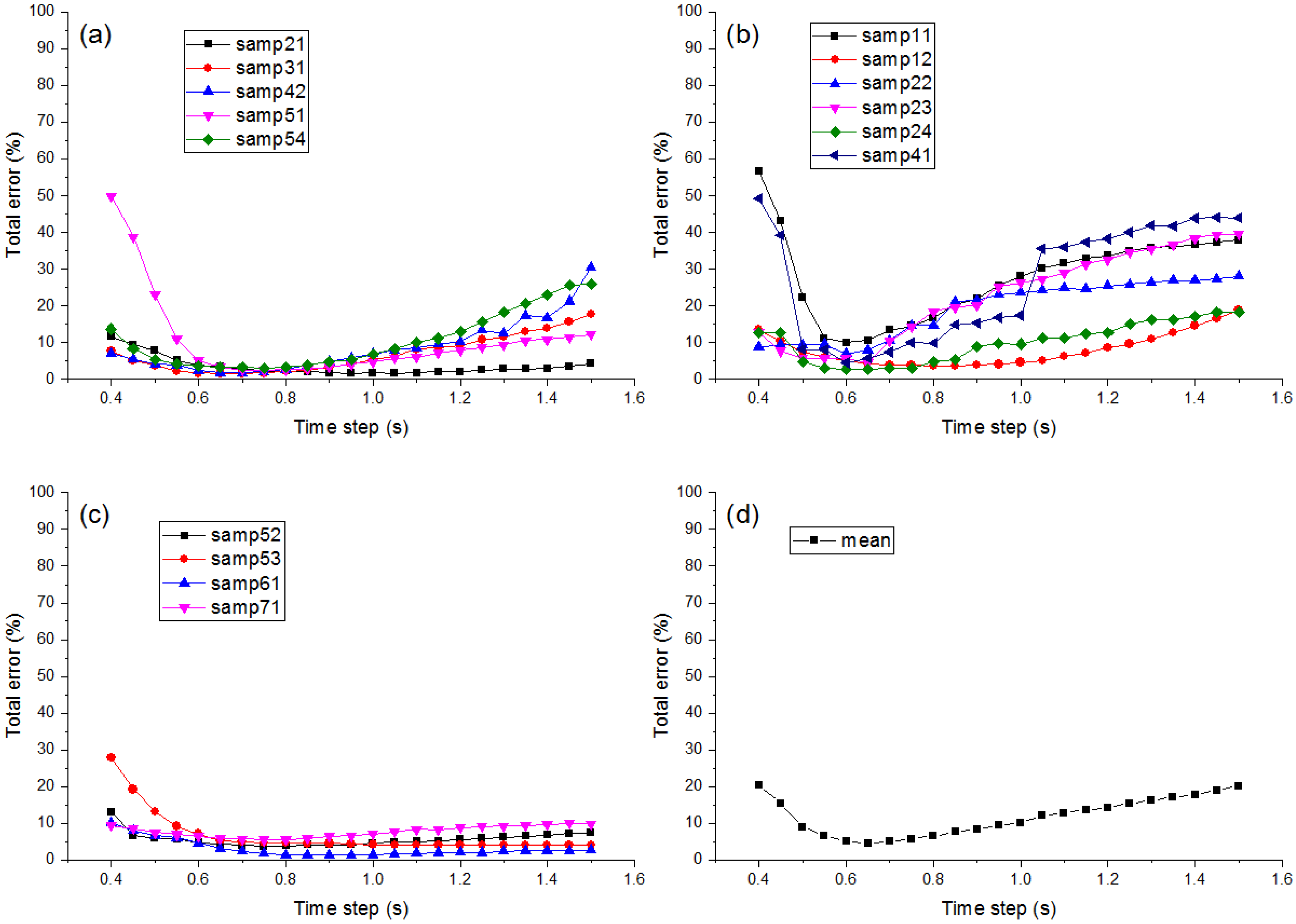
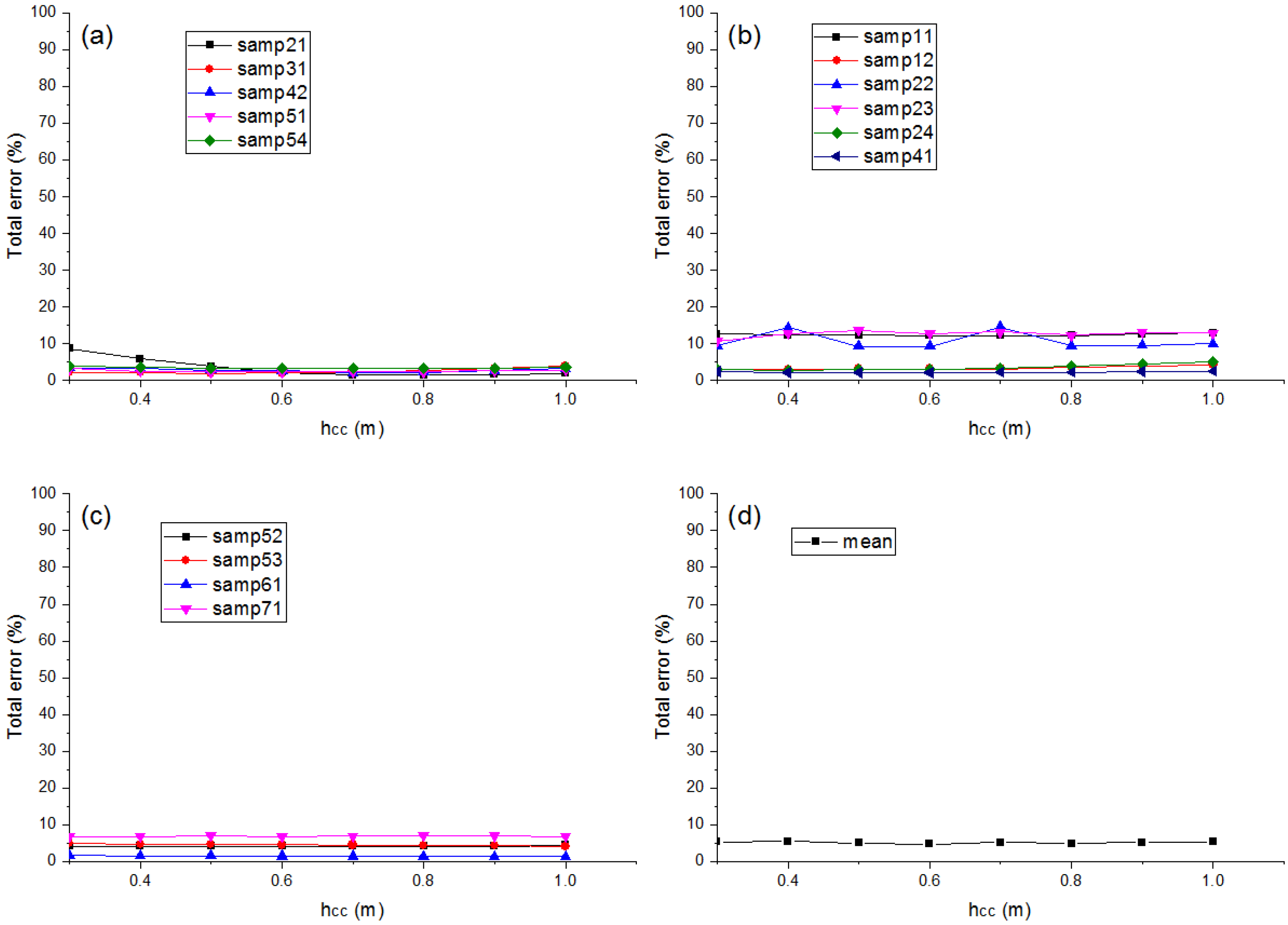
CSF mainly consists of four user-defined parameters: grid resolution (), which represents the horizontal distance between two neighboring particles; time step (), which controls the displacement of particles from gravity during each iteration; rigidness (), which controls the rigidness of the cloth; and an optional parameter steep slope fit factor (), which indicates whether the post-processing of handling steep slopes is required or not.
In addition to these user-defined parameters, two threshold parameters have been used in this algorithm to aid the identification of ground points. The first is a distance threshold () that governs the final classification of the LiDAR points as BE and OBJ based on the distances to the cloth grid. This parameter is set as a fixed value of 0.5 m. Another threshold parameter is the height difference (), which is used during post-processing to determine whether a movable particle should be moved to the ground or not. This parameter is set to 0.3 m for all of the datasets.
5. Conclusions
This research proposes a novel filtering method named CSF based on a physical process. It utilizes the nature of cloth and modifies the physical process of cloth simulation to adapt to point cloud filtering. Compared to conventional filtering algorithms, the parameters are less numerous and are easy to set. Regardless of the complexity of ground objects, the samples were divided into three categories according to the shape of the terrain. Few parameters are needed, and these parameters hardly changed among the three sample categories; only an integer parameter rigidness and a Boolean parameter ST are required to be set by the user. These three groups of parameters exhibit relatively high accuracies for all fifteen samples of the ISPRS benchmark datasets. Another benefit of the CSF algorithm is that the simulated cloth can be directly treated as the final generated DTM for some circumstances, which avoids the interpolation of ground points, and can also recover areas of missing data. Moreover, we have released our software to the public [
35], and we will also release our source code to the research community. We hope that the proposed novel physical process simulation-based ground filtering algorithm could help promote the scientific, government, and the public’s use of LiDAR data and technology to the applications of flood simulation, landslide monitoring, road design, land-cover classification, and forest management.
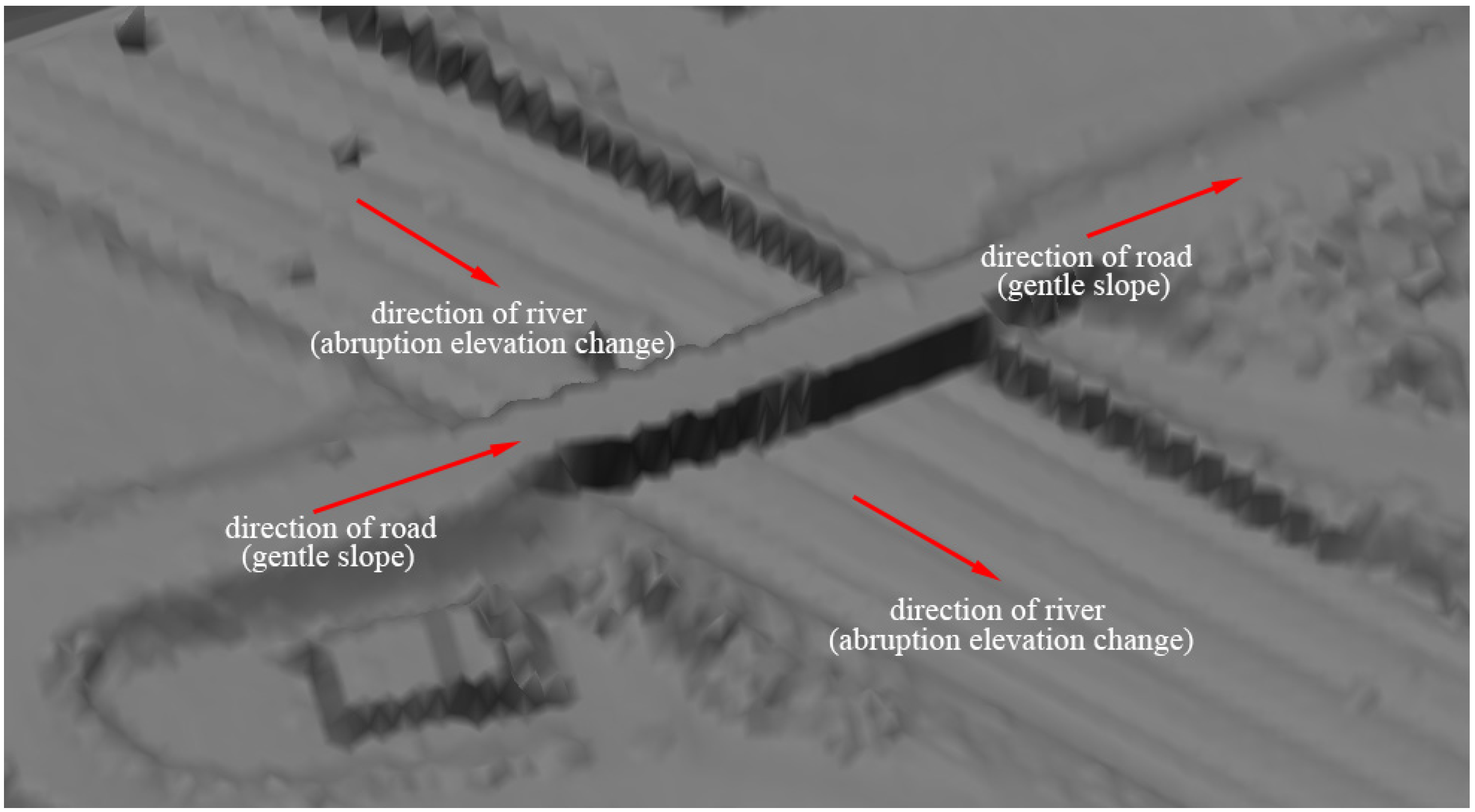
However, the CSF algorithm has limitations as well. Because we have modified the physical processes of particle movement into two discrete steps, the particles may stick to roofs and some OBJ points may be mistakenly classified as BE when dealing with very large low buildings. This process usually produces some isolated points at the centers of roofs, an noise filtering can help to mitigate this problem. Additionally, the CSF algorithm cannot distinguish objects that are connected to the ground (e.g., bridge). In the future, we will try to use the geometry information of LiDAR points or combine optical images (such as multispectral images) to clearly distinguish bridges from roads.


 ,
, 


