1. Introduction
Greenhouse map** via remote sensing is a challenging task due to the fact that the spectral signature of the plastic-covered greenhouse can change drastically [
1,
2,
3,
4,
5,
6]. In fact, different plastic materials with varying thickness, transparency, ultraviolet and infrared reflection and transmission properties, additives, age and colors are used in greenhouse coverings. Moreover, as plastic sheets are semi-transparent, the changing reflectance of the crops underneath them affects the greenhouse spectral signal reaching the sensor [
2].
Over the last decade, greenhouse detection has mainly been addressed by using different pixel-based approaches supported by single satellite data, such as Landsat Thematic Mapper (TM) [
7], Landsat 8 OLI/TIRS [
8], the Terra Advanced Spaceborne Thermal Emission and Reflection Radiometer (ASTER) [
9], IKONOS or QuickBird [
1,
3,
10,
11,
12] and WorldView-2 [
13,
14]. The first paper using object-based image analysis (OBIA) approach for greenhouse detection was published in 2012 by Tarantino and Figorito [
5], in this case working with digital true color (RGB) aerial data. Aguilar
et al. [
6] also applied OBIA techniques on WorldView-2 and GeoEye-1 stereo pairs. Furthermore, a comparison between traditional per-pixel and OBIA greenhouse classification was carried out by Wu
et al. [
15], concluding that the OBIA scheme resulted in a significant improvement.
Monitoring plastic-mulched land cover through per-pixel techniques is attracting a great deal of attention nowadays, particularly in China. In this way, Hasituya
et al. [
16] monitored plastic-mulched farmland by a single Landsat 8 OLI image using spectral and textural features. Working with multi-temporal imagery, Lu
et al. [
17] achieved a very simple but consistent decision tree classifier for extracting transparent plastic-mulched land cover from a very short Landsat 5 TM time series composed by only two images during an agricultural season. They proposed a plastic-mulched land cover index (PMLI) by using the reflectance values of red band (b3) and SWIR1 (b5). Furthermore, large time series of MODIS surface reflectance daily L2G (250 m ground sample distance, GSD) covering the cotton crop period from the 85th day to the 150th day were also used by Lu
et al. [
18] for plastic-mulched land cover extraction. A simple threshold model based on the temporal-spectral features of plastic-mulched land cover in the early stage of a growing season after planting was designed with the number of days (
d) when the normalized difference vegetation index (NDVI) value was larger than a threshold value (
x) as the discriminator. This rule achieved very good results along three different years.
Coming back to greenhouse map**, Aguilar
et al. [
19] went one step further. In this work, the authors addressed the identification of greenhouse horticultural crops that were growing under plastic coverings. To this end, OBIA and a decision tree classifier (DT) were applied to a Landsat 8 OLI time series and a single WorldView-2 satellite image. They used a sample of 694 individual greenhouses whose information such as type of crop, date of planting and date of removal were known. They achieved an overall accuracy of 81.3% in identifying four of the most popular crops cultivated under greenhouse in Almería (Spain). However, in that research, two important issues remained outstanding. On the one hand, Aguilar
et al. [
19] decided to conduct a manual digitizing over the WorldView-2 image in order to obtain the best possible segmentation on their 694 reference greenhouses. On the other hand, the authors did not deal with greenhouse/non-greenhouse pre-classification. In other words, all 694 segments had already been pre-classified as greenhouse.
The multi-resolution segmentation algorithm (MRS) [
20] included in the eCognition Developer software (Trimble, Sunnyvale, California, United States) is one of the most widely used methods to carry out the image segmentation [
21]. It is the first step and a crucial process in the OBIA approach. MRS has already been successfully performed on plastic greenhouses by Tarantino and Figorito [
5] and Wu
et al. [
15]. However, in both cases the three key parameters of MRS (
i.e., scale, shape and compactness) were set up through a systematic trial-and-error approach only validated by visual inspection. At this point, it is important to note that segmentation evaluation plays a critical role in controlling the quality of OBIA workflow. Moreover, among a variety of segmentation evaluation methods and criteria, discrepancy measurement is believed to be the most useful and is therefore one of the most commonly employed techniques in many applications [
22,
23,
24].
The pre-classification of segments as greenhouse or non-greenhouse has to be carried out as a previous step headed up to identify greenhouse horticultural crops growing under plastic coverings. In this way, it is important to point out two critical issues: (1) the shape of the real individual greenhouses should be represented in the best way by the segments to classify; and (2) the classification should be simple, accurate, robust, temporally stable and fast (
i.e., using a small training sample size or even without training). In this way, it could make sense to follow similar approaches to those used by Lu
et al. [
17,
18] but, in this case, through applying an OBIA workflow.
The innovative goal tackled in this paper relies on the combined use of very high resolution satellite data and multi-temporal Landsat 8 OLI imagery, within the context of an OBIA approach, to map and detect individual greenhouses through decision tree classifier. So far, and to the best knowledge of the authors, this is the first research work that deals with this topic using OBIA techniques and Landsat 8 time series. More specific subjects regarding the greenhouse map** method addressed in this work are: (1) identifying the optimal segmentation focused on individual greenhouses by means of segmentation evaluation methods; (2) evaluating the most important and useful features for plastic greenhouse detection (basic spectral information, textural features, several spectral and vegetation indices, seasonal statistics and spectral metric); (3) comparison between the classification accuracies achieved from single satellite imagery and through time series; and (4) determining a simple decision tree temporally stable by using robust threshold values based on Landsat 8 time series and WorldView-2 features for greenhouse classification.
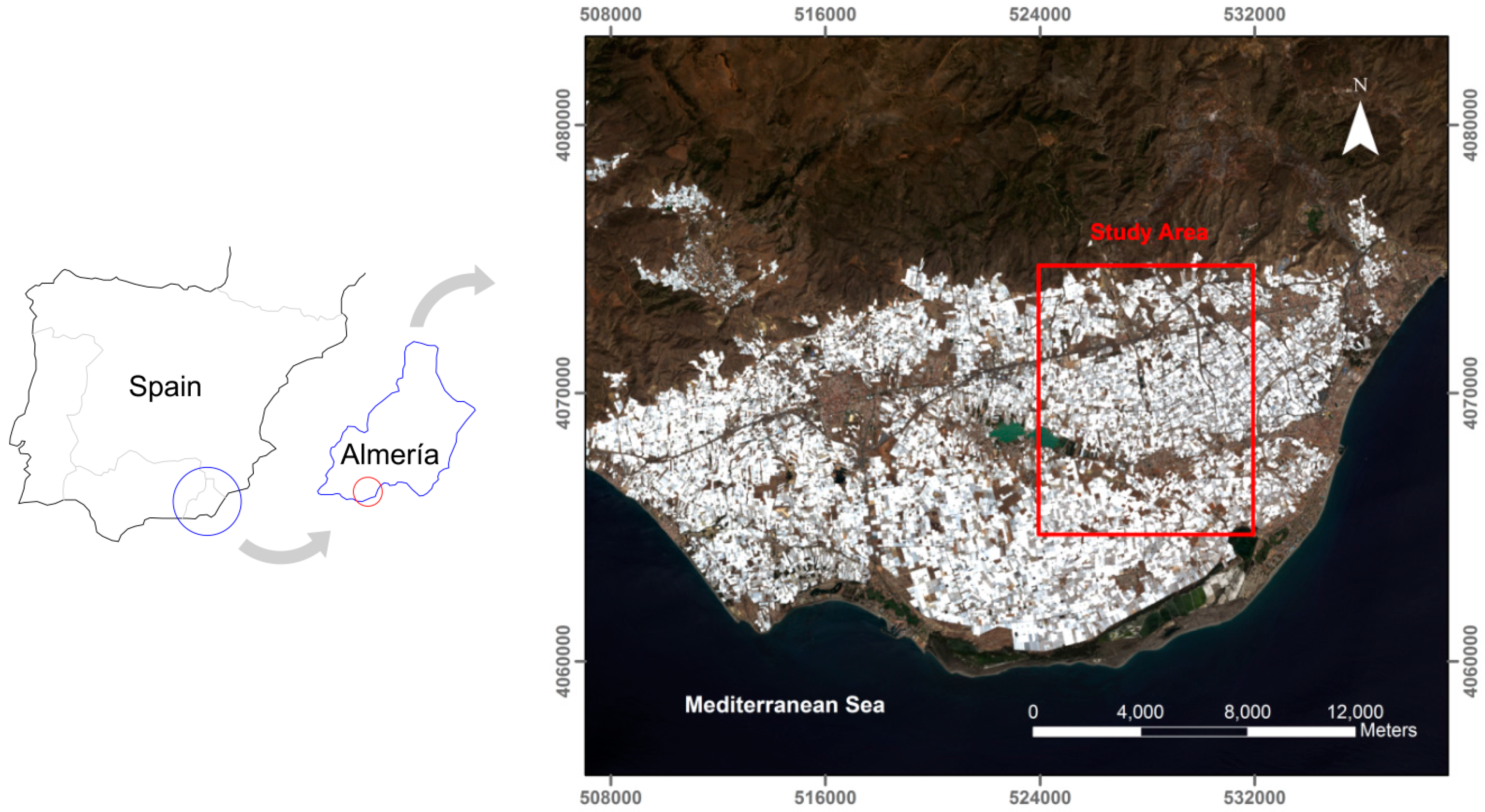
2. Study Area
This investigation was conducted in Almería, southern Spain, which has become the site of the greatest concentration of greenhouses in the world, known as the “Sea of Plastic” or the “Poniente” region. The study area comprises a rectangle area of about 8000 ha centered on the WGS84 geographic coordinates of 36.7824°N and 2.6867°W (
Figure 1).
The types of greenhouse plastic covers in the study area are very variable. The most common materials are polyethylene films (e.g., low density, long life, thermic, with or without additives) and ethylene-vinyl acetate copolymer, also known as EVA. Furthermore, both materials can present different thickness (180 μm or 200 μm) and colors (white, yellow or green). Furthermore, the changing reflectance of the horticultural crops that are growing under semi-transparent plastic coverings during an agricultural season affects the greenhouse spectral signal reaching the sensor. In that sense, the intensive agriculture in Almería was mainly dedicated to tomato, pepper, zucchini, cucumber, eggplant, green bean, melon, watermelon and Chinese cabbage.
3. Datasets
3.1. WorldView-2 Data
WorldView-2 (WV2) is a very high resolution (VHR) satellite launched in October 2009. This sensor is capable of acquiring optical images with 0.46 m and 1.84 m GSD at nadir in panchromatic (PAN) and multispectral (MS) mode, respectively. Moreover, it was the first VHR commercially available 8-band MS satellite: coastal (C, 400–450 nm), blue (B, 450–510 nm), green (G, 510–580 nm), yellow (Y, 585–625 nm), red (R, 630–690 nm), red edge (RE, 705–745 nm), near infrared-1 (NIR1, 760–895 nm) and near infrared-2 (NIR2, 860–1040 nm).
Two single WV2 bundle images (PAN + MS) in Ortho Ready Standard Level-2A (ORS2A) format were acquired for this work. The images over the study area were taken on 30 September 2013 and 5 July 2015. The WV2 image taken in 2013 presented a final product GSD of 0.4 m (PAN) and 1.6 m (MS), while 0.5 m and 2 m were the pixel size for the image taken in 2015. All delivered products were ordered with a dynamic range of 11-bit and without the application of the dynamic range adjustment preprocessing.
From these WV2 ORS2A bundle images, two pan-sharpened images with 0.4 m (2013 WV2 image) and 0.5 m (2015 WV2 image) GSD were attained by means of the PANSHARP module included in Geomatica v. 2014 (PCI Geomatics, Richmond Hill, ON, Canada). The coordinates of seven ground control points (GCPs) and 32 independent check points (ICPs) obtained by differential global positioning system were used at this stage. We used the seven GCPs to compute the sensor model based on rational functions refined by a zero order transformation in the image space (RPC0). A medium resolution 10 m grid spacing DEM with a vertical accuracy of 1.34 m (root mean square error (RMSE)), provided by the Andalusia Government, was used to carry out the orthorectification process. The planimetric accuracy (RMSE2D) attained on the orthorectified pan-sharpened images was of around 0.5 m in both dates.
Furthermore, two MS orthoimages with 1.6 m (2013 WV2 image) and 2 m (2015 WV2 image) GSD containing the full 8-band spectral information were also produced. The same seven GCPs, RPC0 model and DEM were used to attain the MS orthoimage. It is worth noting that atmospheric correction is especially important in those cases where multi-temporal or multi-sensor images are analyzed [
25,
26,
27,
28]. Thus, in this case, and as a prior step to the orthorectification process, the original WV2 MS images were atmospherically corrected by using the ATCOR (atmospheric correction) module included in Geomatica v. 2014. This absolute atmospheric correction algorithm involves the conversion of the original raw digital numbers to ground reflectance values, and it is based on the MODTRAN (MODerate resolution atmospheric TRANsmission) radiative transfer code [
29]. Finally, two atmospherically-corrected WV2 MS orthoimages with a RMSE
2D of around 2.20 m were generated for both dates.
3.2. Landsat 8 Data
The new Landsat 8 (L8) satellite, launched in February 2013, carries a two-sensor payload, the Operational Land Imager (OLI) and the Thermal Infrared Sensor (TIRS). The OLI sensor is able to capture eight MS bands with 30-m GSD: coastal aerosol (C, 430–450 nm), blue (B, 450–510 nm), green (G, 530–590 nm), red (R, 640–670 nm), near infrared (NIR, 850–880 nm), shortwave infrared-1 (SWIR1, 1570–1650 nm), shortwave infrared-2 (SWIR2, 2110–2290 nm) and cirrus (CI, 1360–1380 nm). In addition, L8 OLI presents one panchromatic band (P, 500–680 nm) with 15 m GSD.
Twenty cloud-free multi-temporal L8 OLI scenes type Level 1 Terrain Corrected (L1T) located at the footprint Path 200 and Row 34, each one comprising the whole working area, were downloaded from the U.S Landsat archive. The L8 scenes were taken with a dynamic range of 12 bits from February 2014 to November 2015. These images were really taken as two different time series: One, corresponding to the year 2014, was composed by ten scenes (19 February, 7 March, 24 April, 10 May, 27 June, 14 August, 15 September, 2 November, 18 November and 4 December); and the other ten images belonged to the year 2015 (21 January, 22 February, 10 March, 27 April, 13 May, 30 June, 16 July, 17 August, 18 September and 5 November).
We clipped the original images, both PAN and MS, according to the study area. Bearing in mind that spatial resolutions equal to or better than 8–16 m are recommended by Levin
et al. [
2] to work on greenhouse detection via remote sensing, the fusion of the information of PAN and MS Landsat 8 bands was performed through applying the PANSHARP module included in Geomatica v. 2014. The pan-sharpened images were generated with a GSD of 15 m, 12-bit depth and eight bands (C, B, G, R, NIR, CI, SWIR1 and SWIR2). We applied the ATCOR module (Geomatica v. 2014) to the 20 L8 pan-sharpened images to obtain ground reflectance values. More details about this third step can be obtained from the research published by Aguilar
et al. [
19]. The last process involved the rectification and co-registration of the L8 images. Although all acquired L8 L1T images have been previously orthorectified and corrected for terrain relief [
30], a subsequent co-registration is needed, since an extremely accurate spatial matching among multi-temporal images is crucial in this type of work [
31,
32] for both pixel and object-based image analysis. The pan-sharpened WV2 2013 orthoimage with a GSD of 0.4 m was used as the reference image. Each pan-sharpened L8 image was rectified with this reference image using 50 ground control points evenly distributed over the working area and a first order polynomial transformation. The resulting RMSE
2D for the geometrically-corrected images ranged from 5.29 m to 6.91 m.
5. Results
5.1. Segmentation
In the case of the MRS carried out on the WV2 MS orthoimage taken in September 2013, the minimum value of ED2 (0.11) was reached for the following setting: SP = 49, Shape = 0.3 and Compactness = 0.5. This segmentation was composed of 12,676 objects. Regarding the optimal segmentation for WV2 MS orthoimage from July 2015, 12,975 objects were delimited by using a combination of 34, 0.3 and 0.5 values for SP, Shape and Compactness parameters, respectively. In this case, the ED2 value was 0.29.
5.2. Object-Based Accuracy Assessment
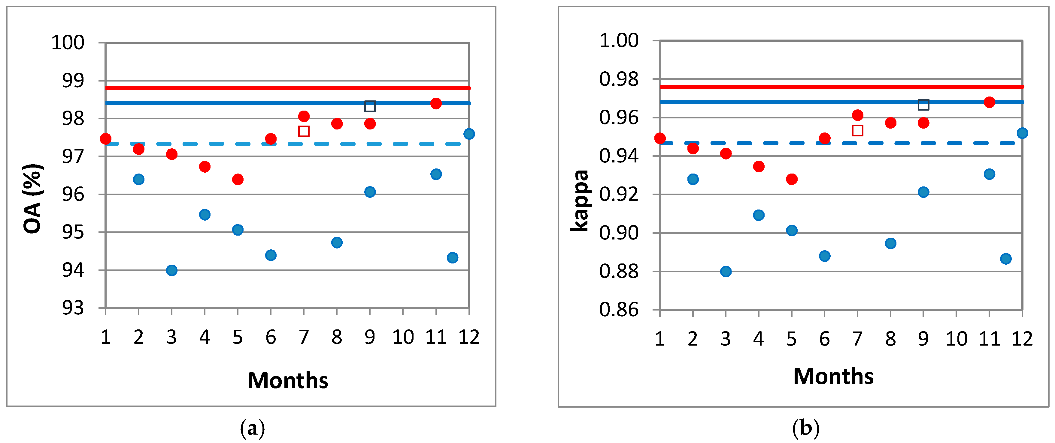
In this section, the goal was to carry out an accuracy assessment based on the 3000 objects per year (1500 for training and the other 1500 for validation). The accuracy results (
i.e., OA, kappa, PA for Greenhouse class (PA_GH) and UA for Greenhouse class (UA_GH)) shown in
Figure 3 come from the confusion matrices finally computed on the validation set (1500 objects) through DT following different strategies:
2014 L8 SI: Single L8 images from 2014 time series (10 images). A blue solid circle represents each accuracy value for each single image from the 2014 time series. In this case, all the features for L8 depicted in
Table 2 were applied on every image.
2015 L8 SI: Single L8 images from 2015 time series (10 images). A red solid circle represents each accuracy value for each single image from the 2015 time series. In this case, all the features for L8 shown in
Table 2 were applied on every image.
2013 WV2: A blue square depicts the accuracy assessment attained from the WV2 image taken in September 2013 using all features shown in
Table 1.
2015 WV2: A red square depicts the accuracy assessment attained from the WV2 image taken in July 2015 using all features shown in
Table 1.
2014 TS: A horizontal blue dashed line depicts the results from the complete L8 2014 time series. In this case, only the statistical seasonal features for the 2014 L8 time series were considered.
2015 TS: A horizontal red dashed line depicts the results from the complete L8 2015 time series. Only the statistical seasonal features for the L8 2015 time series were considered.
2014 WV2 + TS: In this strategy, the features extracted from WV2 2013 were added to the statistical seasonal features for the L8 2014 time series. This strategy is represented as a horizontal blue solid line.
2015 WV2 + TS: The features extracted from WV2 2015 were added to the statistical seasonal features for the L8 2015 time series. A horizontal red solid line depicts this strategy.
It is important to highlight that the DT model computed for 2015 TS and 2015 WV2 + TS strategies were exactly the same. Moreover, only two features were considered in these cases (
i.e., the minimum value of MDI (MIN MDI) and the maximum value of NDVI (MAX NDVI) for 2015 L8 time series). Thus the dashed and solid red lines appear overlapped in
Figure 3. At this point it is noteworthy that our DT classifier was always computed using the prune based on misclassification error as the stop** rule. In the same way as Breiman
et al. [
46], minimal cost-complexity cross-validation pruning was performed to find the “right-sized” tree from amongst all the possible trees. Usually, only two or three split features were selected for each DT.
Regarding the OA and kappa values (
Figure 3a,c), although the accuracies reached from the single L8 images resulted to be very changeable, the results from 2015 single L8 images were overall better than the ones attained from 2014. We have to bear in mind that the segmentation and the class assigned to the 3000 objects were based on the WV2 image taken in September 2013 (
i.e., close but out of 2014). Without any doubt, this fact has come to penalize the final accuracy attained from the single images taken in 2014.
When the statistical seasonal features from the L8 time series of 2014 and 2015 (2014 TS and 2014 TS) were considered, the accuracy was improved, especially in 2015. The OA values were 97.3% and 98.8% for 2014 TS and 2015 TS, respectively. Furthermore, these values turned out to be statistically significant (
p < 0.05) when the confidence intervals were calculated according to [
52].
In the case of WV2 single images, slightly higher OA and kappa values were achieved by using the WV2 2013 image. The OA for WV2 2013 took a value of 98.3%, statistically varying from 97.5% to 98.9% (confidence interval at a significance level of p < 0.05), while in the case of WV2 2015, the OA was 97.7%, with a confidence interval ranging from 96.8% to 98.4%. This tiny and non-significant difference in OA might be due to the different GSD (i.e., 2 m in 2015 and 1.6 m in 2013).
When the information contained in WV2 single images was added to the L8 time series, the accuracy only improved in 2014 while no changes were registered in 2015. In other words, WV2 2015 was not able to add more information to the 2015 TS strategy. In this case, the OA values reached from both strategies were 98.4% and 98.8% for 2014 WV2 + TS and 2015 WV2 + TS, respectively (statistically non-significant differences at p < 0.05).
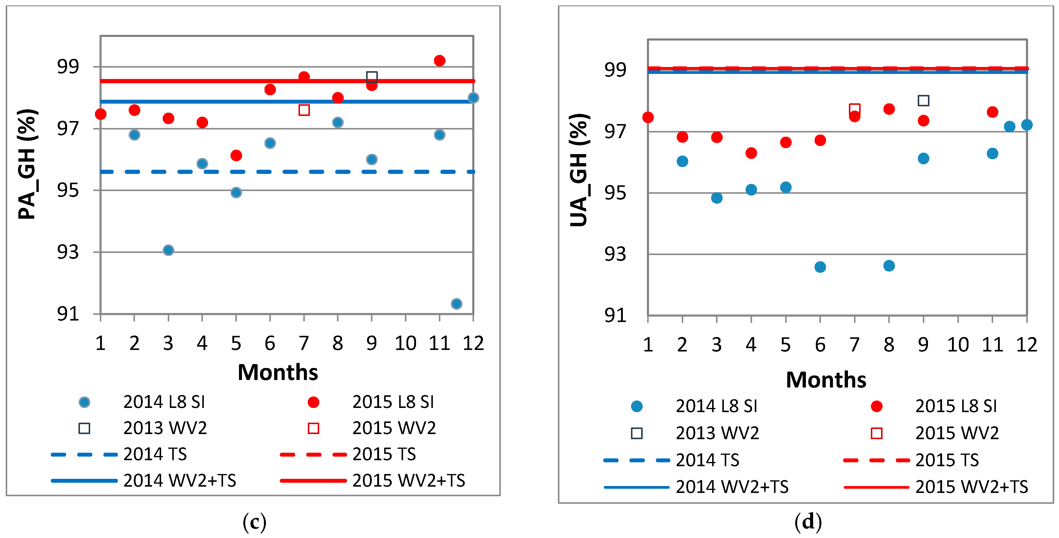
Figure 3c,d shows the Producer’s and User’s accuracy for the Greenhouse class from all the strategies. The PA_GH (
Figure 3c) is an accuracy measure related to error of omission (
i.e., the probability of leaving without classifying an object belonging to the Greenhouse class). The UA_GH indicates the expected error for the Greenhouse class when using the classification map in field or, in other words, the commission error. Both Producer’s and User’s accuracy for the Greenhouse class achieved very good results when WV2 + TS strategy was applied. The reliability of the classification (UA) was very high for the Greenhouse class, with a probability of success greater than 98.9% for both years.
5.3. Importance of Features
The rankings of the 10 most important features used in both WV2 and L8 single images classification are depicted in
Table 3. The ranking for WV2 is achieved by combining the importance of features for the 2013 and 2014 images. In the case of L8, it is performed by merging the importance of features from the 20 single images. For this comparison, the DT projects were carried out using the 3000 objects as training set in order to be more accurate in finding the most important features for each strategy.
The most important features for WV2 single images resulted to be the object-based Mean Coastal and Mean Blue features. These two features were also ranked as very relevant (second and third place) in the case of L8 single images. However, the most significant finding consisted of the MDI feature was selected the first and the most important split feature in 18 out of the 20 DT computed for the single L8 images. Moreover, the threshold or cutting value for this feature was extremely robust with respect to time. In fact, the mean and standard deviation (SD) values of MDI computed thresholds for nine out of 10 images taken in 2014 were 4.33 and 0.10, respectively, while in the case of the 2015 single images, very similar values of 4.38 and 0.08 (mean and SD) were achieved.
Table 4 depicts the most important features for L8 time series when only statistical seasonal features were considered. Three object-based features (MIN MDI, AVG. DIF 8 and DIF SWIR1) stand out over the rest. Regarding the information added by WV2 single images to the L8 time series, only two features (Mean Coastal and Mean Blue) slipped into the top 10 (
Table 4).
5.4. Pixel-Based Accuracy Assessment and Proposed Threshold Model
After analyzing the most relevant features and the most temporally stable cutting values for all the studied cases, a threshold model (TM) for greenhouse detection was proposed. The selected features were MIN MDI and DIF SWIR1 derived from the L8 time series, and the single value of MDI for the WV2 image considered for each year (
Figure 4). It is worth noting that the classifier training phase is not required when using this approach. This TM was again implemented into eCognition to perform the pixel-based accuracy assessment.
Figure 5 shows the OA values for different accuracy assessment schemes studied in this work: (1) object-based using the 3000 reference and meaningful objects as training set and showing the OA confidence intervals (
p < 0.05); (2) pixel-based scheme based on the ground truths manually digitized for the whole study area; and (3) the proposed TM in
Figure 4. It is important to note that in this section we only used the top ten features shown in
Table 3 and
Table 4. As expected, the OA values were always much higher in the case of object-based accuracy assessments than for the pixel-based ones.
Figure 5 depicts these real accuracy results (pixel-based) where the OA values were ranging from 92.3% to 93.8%. When all available information was used (WV2 + TS), the achieved accuracies were 93.8% and 93.1% for 2014 and 2015, respectively. On the other hand, the worst (although quite good) results were attained only using the Landsat data.
A very accurate and temporally stable classification can be achieved by only using the TM, including features from L8 and WV2 (TM L8 + WV2). OA values of 93.0% and 93.3%, and kappa coefficients of 0.856 and 0.861, were attained for 2014 and 2015 datasets, respectively (
Figure 5).
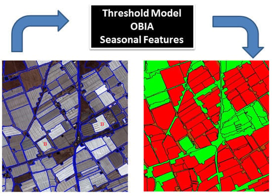
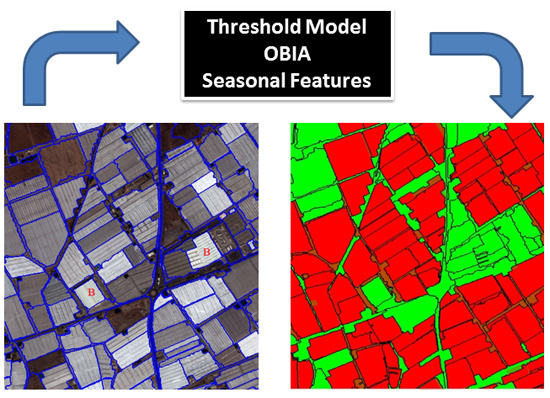
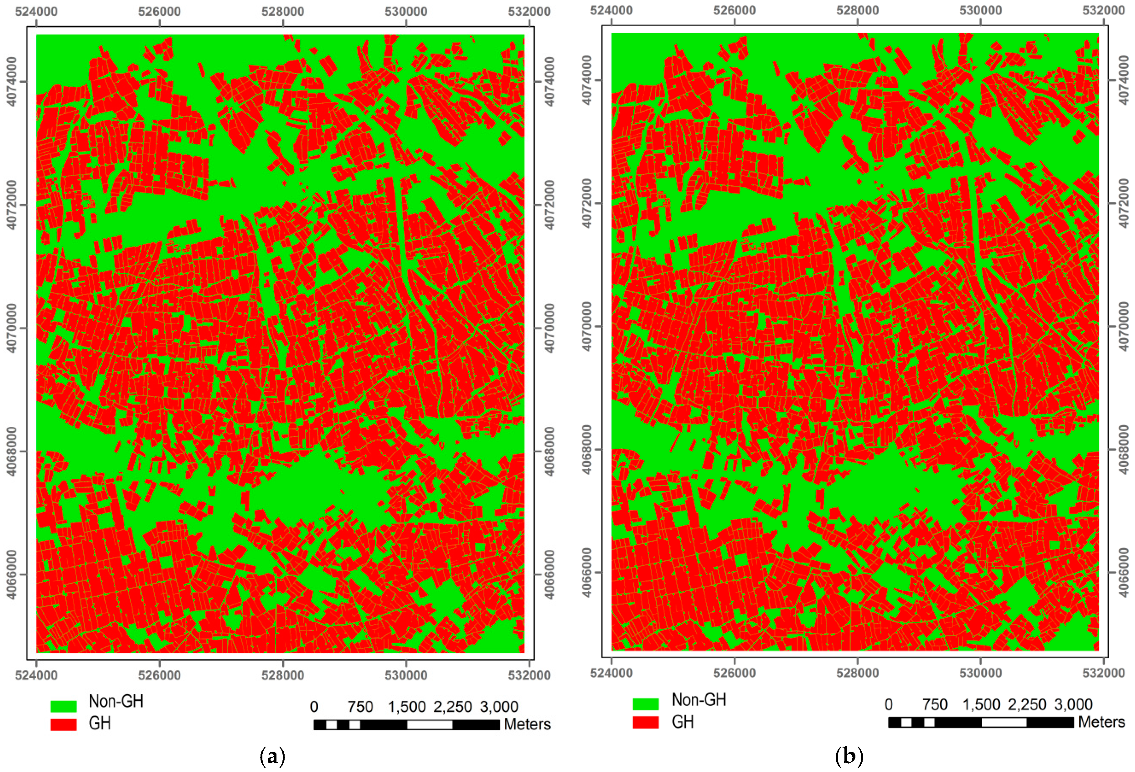
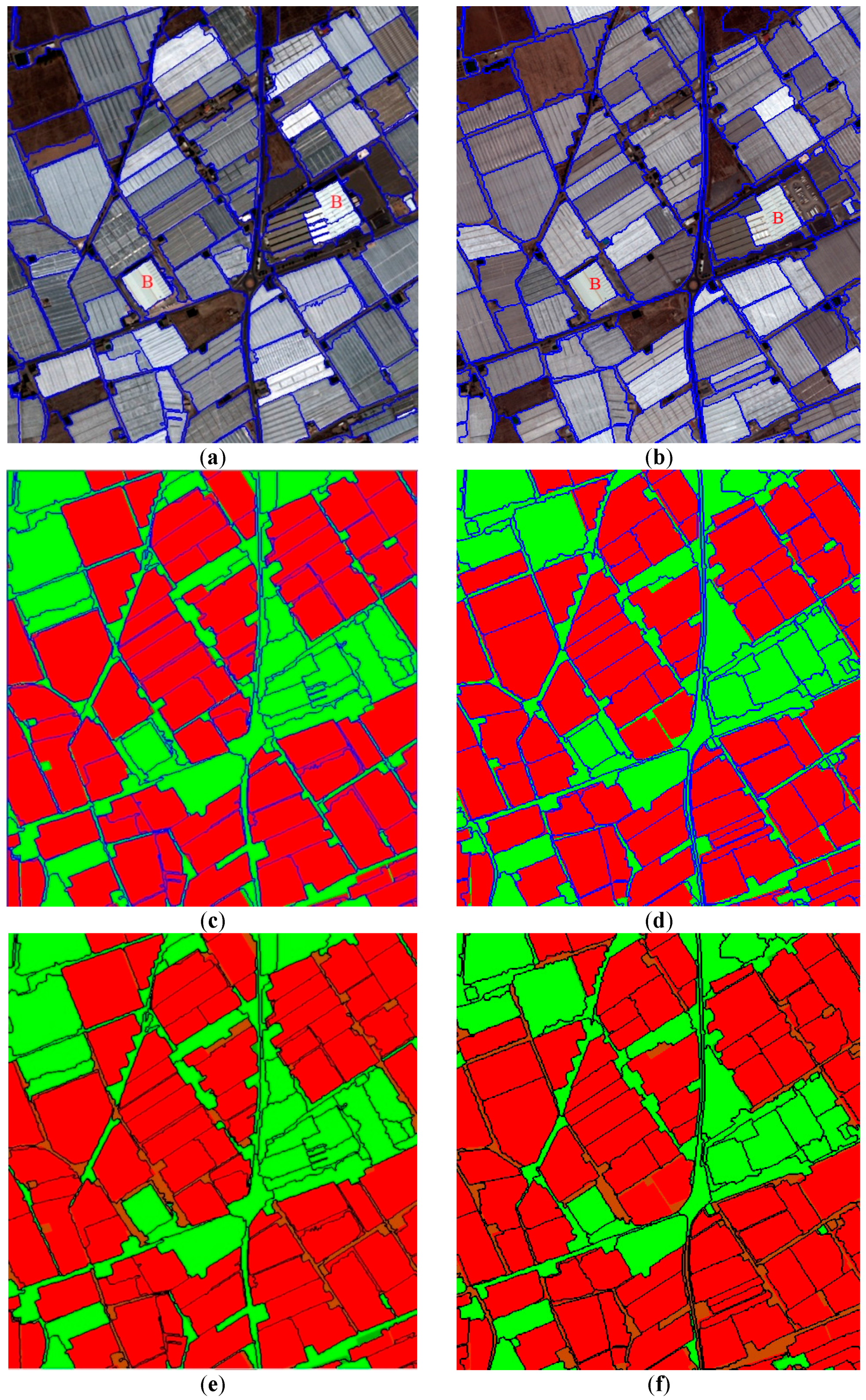
Figure 6 presents the classification process sequence by means of the TM for a detailed area and each year. The first step (
Figure 6a,b for 2014 and 2015) was addressed to obtain the best segmentations from WV2 MS images. In the second step, the two ground truths were manually digitized on the WV2 orthoimages for each year (
i.e.,
Figure 6c for 2013 and
Figure 6d for 2015). The reader can make out that there are few changes between the land cover of both ground truths. After applying the TM through an OBIA approach, a pixel-based comparison was performed between the ground truth and the classification map for each period (
Figure 6e,f).
6. Discussion
The first and crucial step in the OBIA approach is the image segmentation. ED2 metric presented a very good relationship with the visual quality of the greenhouse segmentations. Moreover, this measure was clearly related to SP and Shape (values of Shape should be lower than 0.5), but had no relationship with Compactness. In fact, the weight of this last parameter has been generally set to a fix value of 0.5 [
53,
54]. Although the attained segmentations based on ED2 were of high quality, further works are needed on this issue. Concretely, the optimal combination of bands, the use of VHR pan-sharpened images instead of MS ones and the possible introduction of elevation data should be investigated.
It is important to highlight that in
Figure 3a,b, the accuracy was significantly improved by means of statistical seasonal features from the L8 time series. The seasonal features had already been used by Zillmann
et al. [
55] in grassland map** from multi-sensor image time series. They reported that seasonal statistics should be more consistent over years than snapshot values attained from the original single images.
The texture features based on the Haralick’s matrices tested in both WV2 single images were located at the final positions of the ranking of the importance of features (
Section 5.3), being their contribution for the classification of plastic greenhouses very low. In this sense, Agüera
et al. [
3] reported that the inclusion of texture information in the per-pixel classification of greenhouses from VHR imagery did not improve the classification quality. More recently, Wu
et al. [
15], working with a single Landsat 8 pan-sharpened image within the context of an OBIA approach, found that texture information had very little influence on greenhouse detection. By contrast, the most important feature for greenhouse map** based on single L8 images was the MDI. In fact, a feature specifically aimed at detecting plastic covering such as PLMI [
17] showed much less relevance than MDI.
Figure 5 shows that the OA values were much better when the object-based accuracy assessment was used instead of the pixel-based ones. In that sense, the reader should bear in mind that the 3000 objects selected as ground truth were always meaningful segments. In other words, there were no mixed samples (objects) containing both greenhouse and non-greenhouse land covers. The misclassification problems due to errors in the segmentation stage were also avoided in the case of the object-based accuracy assessment. Moreover, the always very high OA values might undergo small changes as a result of the features selected by the DT model and the objects considered in the evaluation set (see OA in
Figure 3a). Also, no measures were taken to test, reduce and minimize the effect of spatial autocorrelation in the datasets composed of 3000 objects. Thus, spatial autocorrelation may lead to inflated accuracy.
The TM developed in this work and shown in
Figure 4 achieved very accurate and temporally stable classification results. In fact, these accuracy values resulted much more stable over the time than those reported by Lu
et al. [
17,
18] working with time series from Landsat 5 TM and MODIS. The main source of error of the proposed TM was located at elongated objects situated between greenhouses where Non-GH objects were classified as GH (see objects in brown in
Figure 6e,f). According to Wu
et al. [
15], mixed pixels are still commonly present in the pan-sharpened L8 data as a result of the heterogeneity of the landscape and the limitations imposed by the 15 m spatial resolution of the image. This fact is extremely important in the case of the outstretched objects placed between greenhouses.
As it was aforementioned, the use of seasonal statistics from L8 time series allowed us to improve the classification results based only on a single image. For example, the difference of SWIR1 band (DIF SWIR1) seems to be related to the fact that plastic sheets are usually painted white (whitewashed) during summer to protect plants from excessive radiation and to reduce heat inside the greenhouse [
6]. This unique whitewashing management provokes high reflectance values in the SWIR1 bands mainly in the months of July and August, and thus a high value of DIF SWIR1 in the time series (higher than 15 in the TM shown in
Figure 4). Based on this fact, the already reported misclassification between white buildings and plastic greenhouses [
6,
56] can be avoided. In other words, white buildings can show high values of SWIR1 but not very variable over the time.
Figure 6a,b shows two industrial white buildings marked with red letters (B), which are finally well classified thanks to the DIF SWIR1 threshold. Regarding the MDI object-based feature computed from both WV2 and L8 sensors, it turned out to be the most important feature related to plastic greenhouse detection. Moreover, it showed extreme robustness over time. All of the single L8 images presented an almost constant threshold value of MDI of around 4, while for WV2 single images the MDI cutting value was located between 0.5 and 0.55. Without any doubt, this has been one of the most important findings in this work. Moreover, the discriminatory power of the MDI was improved by using the MIN MDI in the case of L8 time series.
MDI was developed to take advantage of the information latent in the shape of the reflectance curve that is not available from other spectral indices [
44]. This spectral metric has been able to discriminate between GH and Non-GH from an OBIA approach. However, we have detected a few confusion problems mainly with building class. These misclassification errors can be solved using seasonal statistic features. Really, in this paper, we are only scratching the surface, so further investigations should be needed in order to understand the relationship between the MDI and plastic greenhouses. Furthermore, the threshold values of MDI or MIN MDI for this study were obtained from the same study area and should be further tested in other greenhouse areas and even using other sensors.
7. Conclusions
In this work, a new and accurate approach to address the problem of greenhouse map** was presented. It consisted of the combined use of VHR satellite data (W2 Multispectral imagery in this case) and L8 OLI pan-sharpened time series within the context of an OBIA approach. Additionally, the classification results were assessed for two different years in order to test the desirable temporal stability.
The first stage was focused on achieving the optimal segmentation for individual greenhouses by using MRS algorithm on the single WV2 MS orthoimages. In this sense, ED2 metric presented a very good relationship with the visual quality of the greenhouse segmentations so allowing select the main MRS parameters (i.e., Scale, Shape and Compactness) for each WV2 orthoimage.
In the second step, the DT classifier was selected to determine the best object-based features for greenhouse map** and estimate their more adequate threshold values. Many strategies were carried out involving different combinations of single images from L8 and WV2. L8 time series were also tested allowing use seasonal statistics, which significantly improved the accuracy attained through single L8 images.
Finally, a spectral metric feature, never before tested in greenhouse detection or in OBIA approaches, turned out to be the most important characteristic related to plastic greenhouse detection for both WV2 and L8 sensors. Moreover, it showed an extremely robustness over the time. In fact, a TM only comprising three features was proposed for the two considered years. The first two selected features, the minimum value of MDI (MIN MDI) and the difference between the maximum and minimum value of SWIR1 (DIF SWIR1), were derived from the L8 time series. The last one was the single value of MDI for the WV2 image. In this sense, it was proven that a very accurate and temporally stable classification of individual greenhouses can be achieved by only using the proposed TM in which the classifier training phase is not required. Very stable over the time OA values of 93.0% and 93.3% were attained for 2014 and 2015 datasets, respectively.
These findings are quite promising, though they should be further contrasted working on other greenhouse or plastic-mulched land cover locations and also testing others medium spatial resolution satellites such as the recently launched Sentinel-2.


 ,
, 


