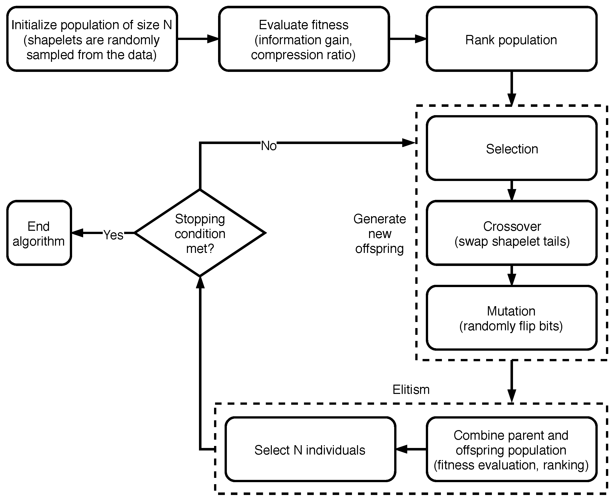
3.2.1. Using NSGA-II to Extract Time Series Shapelets
Evolutionary algorithms have already been profitably used in different phases of the decision tree learning process [
52]. In order to describe how we adapted NSGA-II for the task of shapelet generation, in the following we will discuss:
how the population (i.e., potential solutions) is represented and how it is initialized;
how the crossover and mutation operators are defined;
which fitness function and constraints are used;
which decision method is followed to select a single solution from the resulting front, given that, as we shall see, we are considering a multi-objective setting.
Differently from the majority of previous works, in our solution we do not require shapelets to be part of any training time series: once they are initialized with values taken from the time series data, they may evolve freely through the generations. As for the implementation of the evolutioary algorithm, we relied on the jMetal framework [
53].
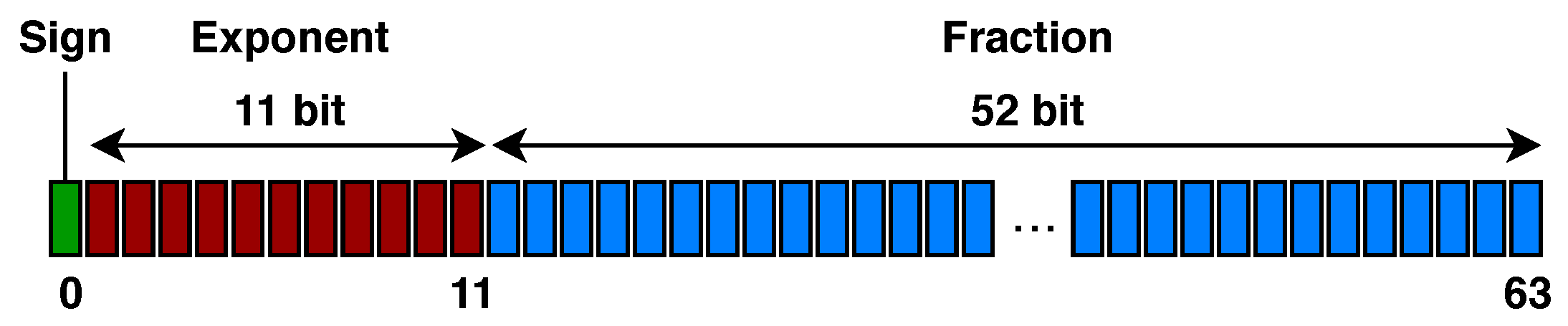
Representation of the Solutions and Initial Population. In order to make it easier for us to define the
mutation operator, we decided to represent each shapelet in the population by an ordered list of binary arrays, each one of them encoding a floating point value in
IEEE 754 double-precision 64 bit format (see
Figure 5): the first, leftmost bit establishes the sign of the number, the following 11 bits represent the exponent, and the remaining 52 bits encode the fraction.
As for the initialization of the population, the step is performed on each instance as follows: first, a time series is randomly selected from the dataset; then, a begin and an end index are randomly generated. The shapelet corresponds the portion of the time series that lies between the two indexes.
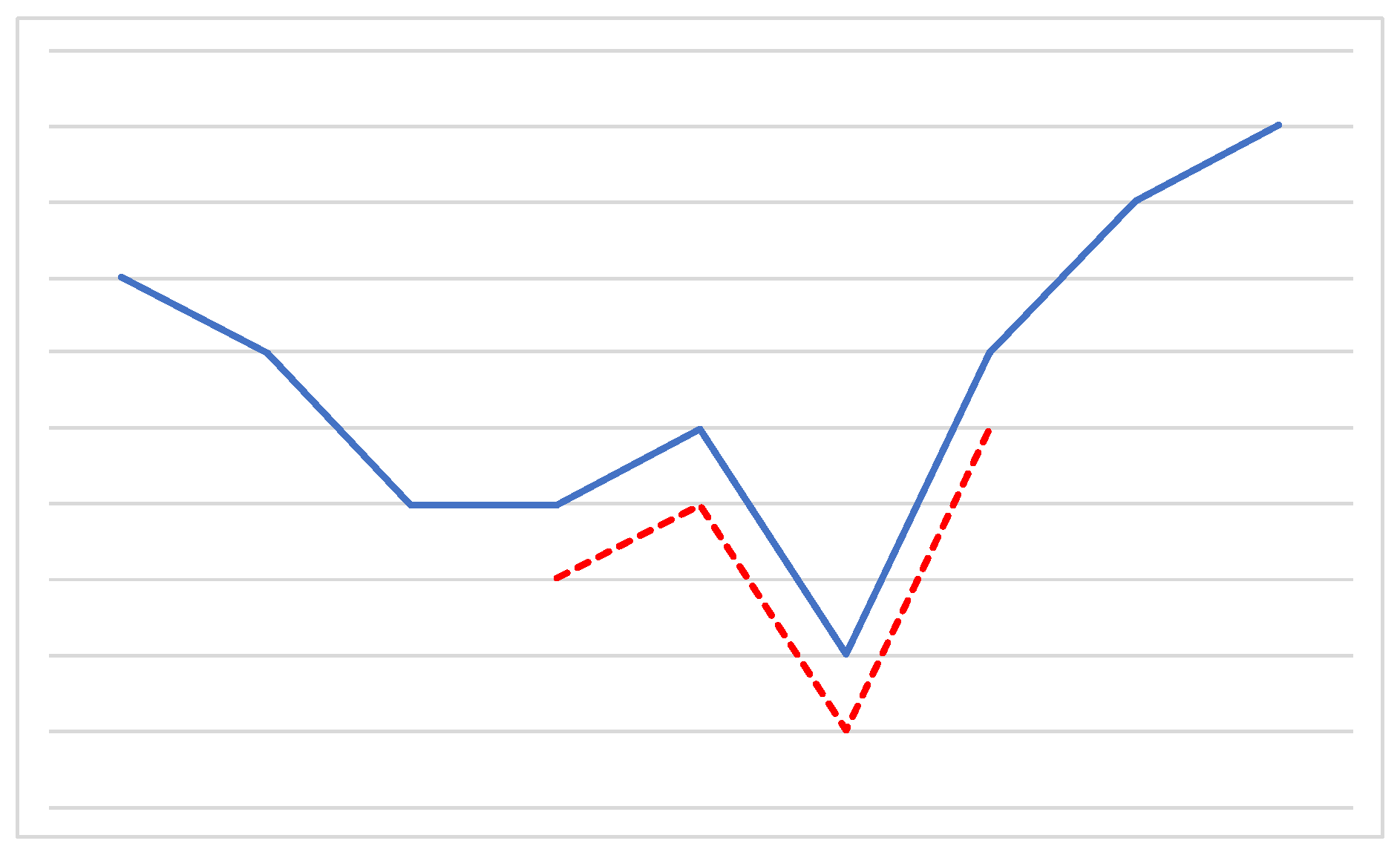
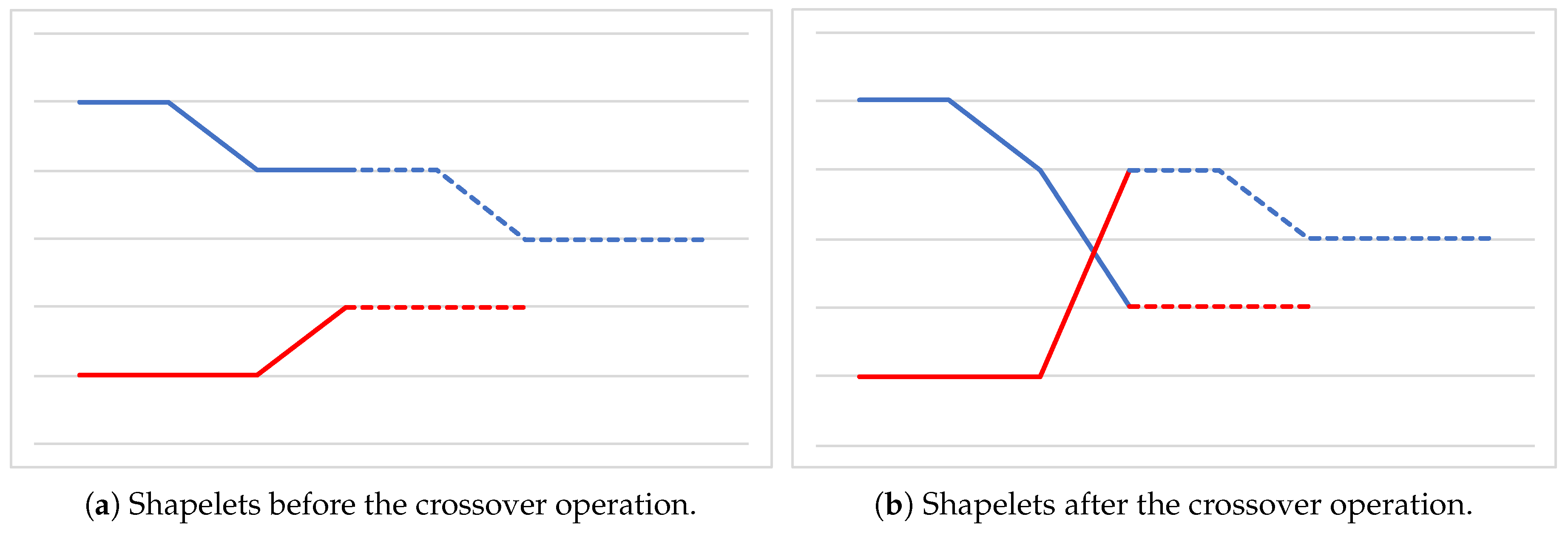
Crossover Operator. As for the crossover operator, we rely on an approach similar to the
single-point strategy [
29]. Given two parent solutions, that is, two lists of binary arrays, a random index is generated for each of them. Such indexes represent the beginning of the
tails of the two lists, that are then swapped between the parents, generating two offspring.
Figure 6 graphically represents the crossover operation, where the two indexes happen to have the same value. Observe that, in general, the two offspring may have a different length with respect to those of the two parents.
Mutation Operator. A properly designed mutation operator should not try to improve a solution on purpose, since this would bias the evolution process of the population. Instead, it should produce random, unbiased changes in the solution components [
29]. In the present approach, mutation is implemented by randomly flip** bits in the binary array representation of the elements composing the shapelet. Since we rely on the IEEE notation, the higher the index in the array, the less significant the corresponding bit. Taking that into account, we set the probability of flip** the
ith bit to be
, where
is the overall mutation probability, governed by the
mutationP parameter. Intuitively, by employing such a formula, we effectively penalize flip** the most significant bits in the representation, avoiding sharp changes in the values of the shapelets that might interfere with the convergence of the algorithm to a (local) optimum. Finally, when randomly flip** the bits leads to non-valid results (
NaN in the IEEE 754 notation), we simply perform a further random flip in the exponent section of the binary array.
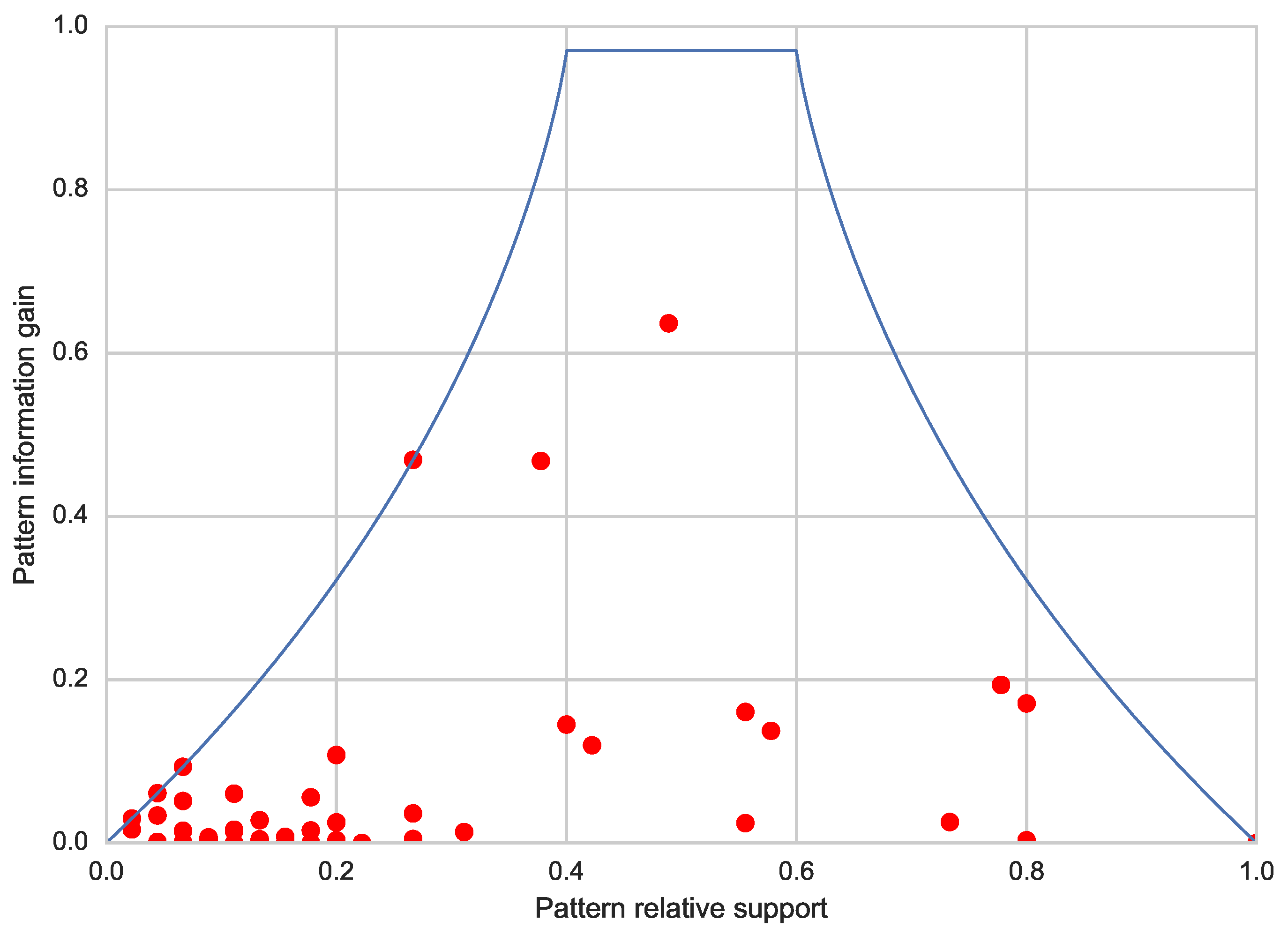
Fitness Function. In our implementation, we make use of a bi-objective fitness function. The first one is that of maximizing the information gain (IG) of the given shapelet, as determined on the training instances belonging to the specific tree node: observe that such a measure corresponds to the normalized gain, since a split over a shapelet is always binary. To calculate the IG of a shapelet, first its minimum Euclidean distance with respect to every time series is established, by means of a sliding window approach. Then, the resulting values are dealt with following the same strategy as the one used by C4.5/J48 for splitting on numerical attributes (see, for instance, [
1]). Observe that, in principle, one may easily use any other distance metric in the objective.
The second objective is that of reducing the
functional complexity [
35] of the shapelet, so to fight against undesirable overfitting phenomena that might occur if considering only the first objective. To do so, we make use of the well-known
Lempel-Ziv-Welch (LZW) compression algorithm [
54]: first, we apply such an algorithm to the (decimal) string representation of the shapelet, and then we evaluate the ratio between the lengths of the compressed and the original strings. Observe that such a ratio is typically less than 1, except for very small shapelets, in which compression might actually lead to longer representations, given the overhead of the LZW algorithm. Finally, NSGA-II has been set to minimize the ratio, following the underlying intuition that “regular” shapelets should be more compressible than complex, overfitted ones. As a side effect, also extremely small (typically singleton) and uninformative shapelets are discouraged by the objective.
Given the fact that we use a bi-objective fitness function, the final result of the evolutionary process is a set of non-dominated solutions.This turns out to be an extremely useful characteristic of our approach, considering that different problems may require different levels of functional complexities of the shapelets in order to be optimally solved. As we shall see, one may easily achieve a a trade-off between the two objectives by simply setting a parameter. It is worth mentioning that we also tested other fitness functions, inspired by the approaches described in
Section 2.3. Among them, the best results have been given by:
an early-stop** strategy inspired by the separate-set evaluation presented in [
34]. We first partition the training instances into two equally-sized datasets. Then, we train the evolutionary algorithm on the first subset, with a single-objective fitness function aimed at maximizing the information gain of the solutions. We use the other dataset to determine a second information gain value for each solution. During the execution of the algorithm, we keep track of the best performing individual according to the separated set, and we stop the computation after
k non improving evolutionary steps. Finally, we return the best individual according to the separated set;
a bootstrap strategy inspired by the work of [
33]. The evolutionary algorithm evaluates each individual on 100 different datasets, built through a random sampling (with replacement) of the original dataset. Two objectives are considered: the first one is that of maximizing the average information gain of the shapelet, as calculated along the 100 datasets, while the second one tries to minimize its standard deviation, in an attempt to search for shapelets that are good in general.
As a matter of fact, both these strategies exhibited inferior accuracy performance than the previously discussed solution. While for the first approach this might be explained by the fact that it greatly reduces the number of training instances (a problem that is exacerbated in the smallest nodes of the tree), the reason behind the poor performance of the second one is still unclear, and deserves some further attention.
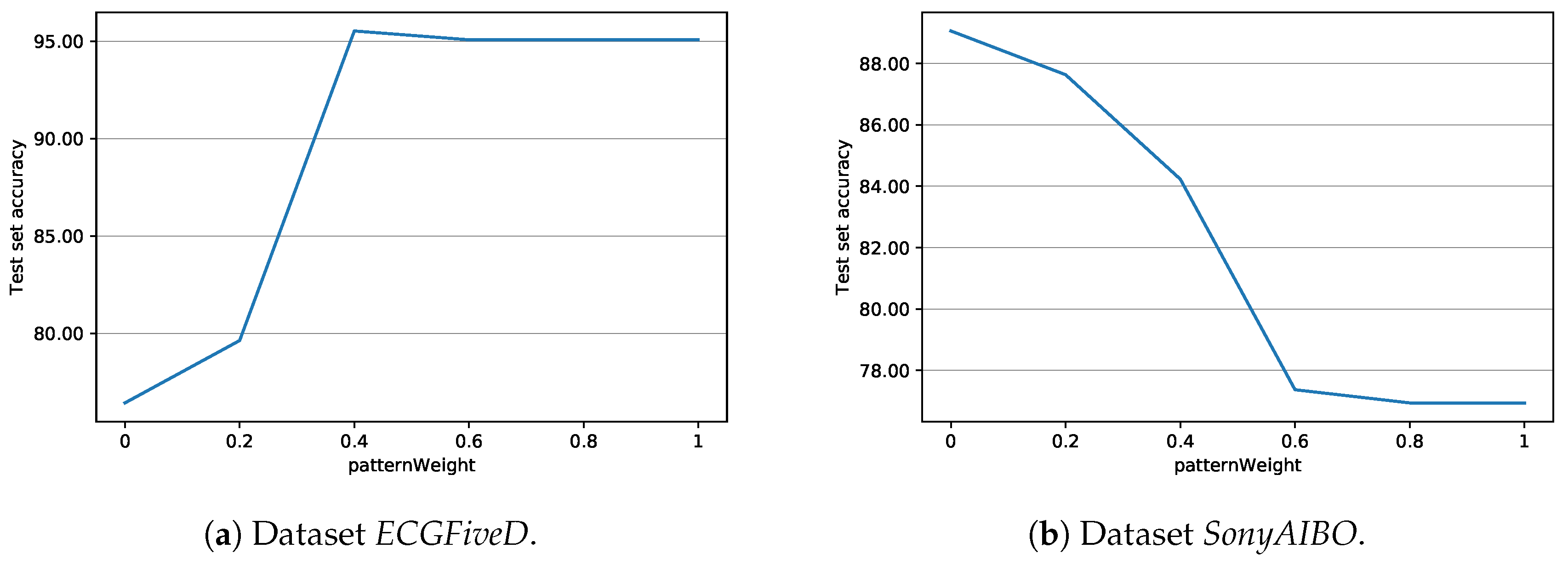
Decision Method. In order to extract a single shapelet out from the resulting front of Pareto-optimal solutions, we evaluate each individual with respect to the following formula:
where
is a weight that can be customized by the user (by the
patternWeight parameter),
is the compression ratio of the shapelet, and
is the information gain of the shapelet, both divided by the respective highest values observed in the population. The solution that minimizes the value of such a formula is selected as the final result of the optimization procedure, and is returned to the decision tree for the purpose of the splitting process. Intuitively, large values of
W should lead to a highly accurate shapelet being extracted (at least, on the training set). Conversely, a small value of
W should result in less complex solutions being selected. Note that the approach is quite similar to the one we used to handle sequential data: in fact, this allows us to seamlessly rely on the same weight
W in both cases.
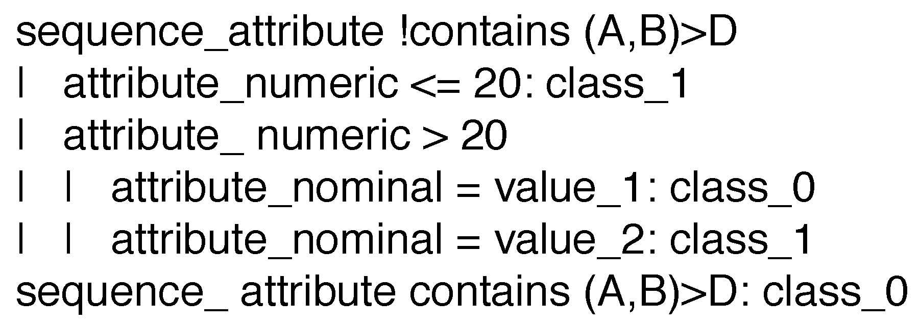
3.2.2. Adapting J48 to Handle Time Series Data
Consider now the execution of J48SS on time series data, concerning the tree growing phase. Algorithm 1 illustrates the main procedure that is used during the tree construction phase: it takes a node as input, and proceeds as follows, starting from the tree root. If the given node already achieves a sufficient degree of purity (meaning that almost all instances are characterized by the same label), or any other stop** criteria is satisfied, then the node is turned to a leaf; otherwise, the algorithm has to determine which attribute to rely on for the split. To do so, first it considers all classical attributes (categorical and numerical), determining their
normalized gain value (see
Section 3.1.2), according to the default C4.5 strategy. Then, it centers its attention on string attributes that represent sequences: VGEN is called in order to extract the best
closed frequent pattern, as described in
Section 3.1. Then, for each string attribute representing a time series, it runs NSGA-II with respect to the instances that lay on the node (see the details presented in the remainder of the section), obtaining a shapelet. Such a shapelet is then evaluated as if it was a numerical attribute, considering its Euclidean distance with respect to each instance’s time series (computation is sped up by
subsequence distance early abandon strategy [
39]), and thus determining its normalized gain value, that is compared to the best found one. Finally, the attribute with the highest normalized gain is used to split the node, and the algorithm is recursively called on each of the generated children.
| Algorithm 1 Node splitting procedure |
- 1:
procedurenode_split(node) - 2:
if NODE is “pure” or other stop** criteria met then - 3:
make NODE a leaf node - 4:
else - 5:
- 6:
- 7:
for each numeric or categorical attribute a do - 8:
get information gain of a - 9:
if then - 10:
- 11:
- 12:
for each sequential string attribute s do - 13:
get best frequent pattern in s - 14:
if then - 15:
- 16:
- 17:
for each time series string attribute t do - 18:
get shapelet in t using NSGA-II - 19:
if then - 20:
- 21:
- 22:
split instances in NODE on - 23:
for each child_node in children_nodes do - 24:
call NODE_SPLIT(child_node) - 25:
attach child_node to NODE - 26:
return NODE
|
As for the input parameters of the procedure for the shapelet extraction process, they are listed in
Table 2. With the exception of
patternWeight, which determines the degree of
complexity of the shapelet returned to the decision tree by NSGA-II (see Algorithm 1), they all regulate the evolutionary computation:
crossoverP determines the probability of combining two individuals of the population;
mutationP determines the probability of an element to undergo a random mutation;
popSize determines the population size, i.e., the number of individuals;
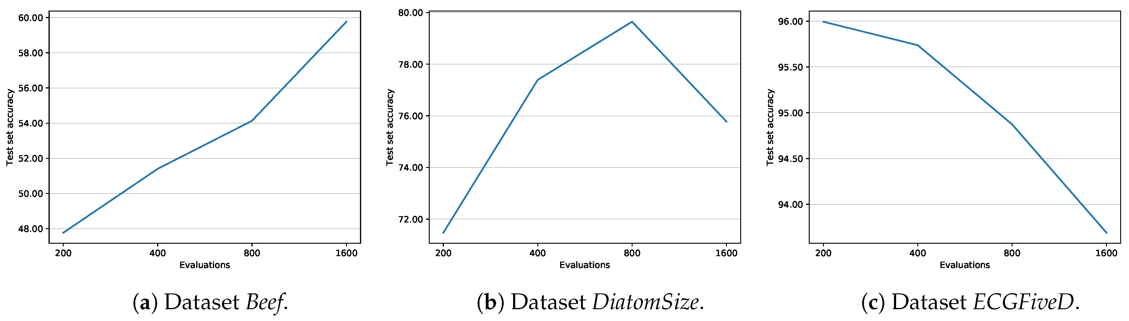
numEvals establishes the number of evaluations that are going to be carried out in the optimization process.
Of course, when choosing the parameters, one should set the the number of evaluations (numEvals) to be higher than the population size (popSize), for otherwise high popSize values, combined with small numEvals values, will in fact turn the evolutionary algorithm behaviour to a blind random search. Each parameter comes with a sensible default value that has been empirically established. However, a dedicated tuning phase of patternWeight and numEvals is advisable to obtain the best performance.


