1. Introduction
The widespread conversion of natural forests into woody plantation crops in tropical regions can strongly impact regional carbon budgets and water resources [
1,
2,
3]. In Southeast Asia, one of the major drivers of such land-use change has been the demand for rubber [
4,
5]. Consequently, this land-use type occupies relatively large territories in Southeast Asia and the world. Although rubber trees have been cultivated for several decades [
6,
7], little is known about how monocultures of these trees differ from natural forests in terms of exchange of carbon dioxide and water vapor with the atmosphere. There exists limited observational data on leaf-level physiology (e.g., photosynthetic capacity, stomatal conductance) [
8,
9] ecosystem-scale exchanges of gases, water, and energy in rubber plantations [
10,
11]. Consequently, the temporal and regional variability of such properties for these ecosystems remains unknown.
Understanding carbon and water cycling processes at the site level is the first step in determining how rubber plantations’ expansion impacts carbon sequestration, ecosystem services, and other environmental variables. While data from site-level studies that utilize field-based techniques are essential for examining how carbon and water cycling processes are influenced by land-use conversion to rubber plantations [
12,
13], there are inherent shortcomings when extrapolating short-term site-level observations to longer temporal and larger spatial scales. Therefore, ecosystem modeling that represents a mechanistic understanding of ecosystem function and processes is often used [
14]. For example, Kumagai et al. [
15] developed a soil–vegetation–atmosphere transfer model for rubber plantations (SVAT-rubber). They examined how canopy structure in the model affected carbon and water fluxes in central Cambodia, while Yang et al. [
16] used the Land Use Change Impact Assessment model to simulate rubber (LUCIA) and investigated how high altitudes and planting densities influenced the modeled biomass and latex yield of rubber plantations. It is worth noting that the former study considered only one site, and therefore their results could be site-specific. In contrast, the latter study did not properly simulate rubber’s canopy development.
Some statistical models have been developed to predict suitable areas for growing rubber plantations [
17,
18,
19]. For example, Liu et al. [
17] investigated the impacts of future climate change on the suitability of rubber plantations in China by utilizing five main climatic factors. Their results showed that the rubber plantation would have a trend of expansion to the north in 2041–2080. Ray et al. [
19] used an ecological niche model to analyze the present and potential future distribution of rubber trees in two biogeographically distinct regions of India, i.e., the Western Ghats (WG) and Northeast (NE). Ray et al. [
19] found more areas would be suitable for rubber tree plantation in the NE region, whereas further expansion would be limited in the WG region under the projected climate scenario for 2050. Using a statistical regression model (SRM), Lang et al. [
20] disentangled the links between soil water content, soil texture, and mineral nitrogen in rubber plantations and assessed the impacts of land-use change on methane flux. Land surface models are also increasingly adopted to investigate the impact of land-use change on carbon and energy fluxes at various temporal and spatial scales [
21,
22,
23]. To simulate vegetation dynamics and interactions with the soil and atmosphere, land surface models usually reduce intra- and interspecies vegetation diversity into a few plant functional types (PFTs), defined by the key physiological and morphological characteristics of specific plant groups and their essential ecological functions [
24]. There are several advantages in using a land surface model to investigate terrestrial ecosystem processes and the impact of land-use change, including: (1) an examination of diurnal, seasonal, and longer-term changes in carbon, water, and energy cycling across spatial scales [
25,
26]; (2) the identification of crucial and sensitive model parameters [
26,
27]; and (3) assessing historical and future climate change impacts on natural and agroecosystem functioning [
23,
28].
Phenology is an important aspect of any PFT in land surface models, for it regulates the timing of leaf onset and offset [
29,
30], the rate of leaf litterfall [
31], and associated stomata-level processes of water and carbon exchanges in response to varying environmental conditions. The phenology of rubber varies across regions, making its parameterization challenging in models applied to the global scale. The rubber tree (
Hevea brasiliensis) is native to the Amazon rainforest [
32] but cultivated throughout the tropics. Although native rubber is evergreen, it can turn to semideciduous (facultative deciduous) in other tropical [
33] and subtropical environments [
7,
10]. In locations with a pronounced dry season, the leaf fall period is short, and refoliation occurs before the start of the rainy season [
34]. Sustained period of reduced daylength could also trigger leaves to fall in rubber plantations [
35,
36]. Moreover, the leaf phenology of rubber is associated with reproduction. Empirical data show rubber trees increase their leaf litterfall rates when they allocate carbon to produce fruits [
37]. This study introduces and simulates rubber utilizing an advanced land surface model, the Community Land Model version 5 [
26,
38]. CLM5 currently includes fourteen natural vegetation and eight crop PFTs, which allow an adequate description of the main variety of global vegetation phenology (e.g., evergreen, stress–deciduous, seasonal–deciduous, and annual single-season crops), morphology (e.g., needle-leaf and broadleaf trees, shrubs, and grasses) and physiology (C3 and C4 photosynthesis, carbon and nitrogen allocation, etc.) across different climate zones [
39]. However, perennial tree crops are not yet included, even though they occupy an increasing land surface in tropical regions [
4]. This is partly because of the limited data available for the parameterization of critical processes. The development of rubber as a PFT in CLM5 will help investigate how the rubber plantations respond to nitrogen fertilization rates and extreme climate events (e.g., those caused by El Nino–Southern Oscillation). Rubber PFT in CLM5 can also simulate the spatial distribution of carbon and water fluxes at regional and continental scales. Since rubber is a facultative deciduous species; that is, it is a partial deciduous species which is evergreen most of the year; it is useful to simulate rubber using baseline values of tropical evergreen PFT or tropical deciduous PFT and compare the model outputs with our newly developed rubber PFT with reference to empirical field measurements of rubber productivity and ecosystem functions.
The main objective of this current modeling effort is to develop a new rubber PFT in CLM5 (and introduce rubber-specific functions) using data from a rubber clone in Jambi, Indonesia. We synthesized the data collected in several short-term field surveys and an intensive one-year measurement campaign in smallholder rubber plantations in Jambi, Indonesia, and subsequently used these data for model calibration. We also compared our modeling results with data from previous rubber modeling studies.
2. Methods
2.1. Study Sites
The main study site used in this research is located in the lowlands of Jambi province, Sumatera, Indonesia (2° S, 103° E, 40–70 m above sea level), with site selection reflecting the fact that a relatively large part of the lowlands in Jambi province was converted to oil palm and rubber plantations in the previous two decades [
6,
40]. The region’s climate is tropical maritime [
41], with mean annual temperature and mean annual precipitation in Jambi averaging 26.7 ± 1.0 °C and 2235 ± 385 mm, respectively [
6]. The dry season usually starts in May (~130 mm per month) and lasts until September (~20 mm per month), while the rainy season is between October and April.
Measurements were performed in the Harapan landscape within the Jambi province, characterized by loam Acrisol soils [
12], and sites are located about 80 km southwest of Jambi City. Within the landscape, four rubber plantations were chosen and within each plantation, a 50 m × 50 m plot was established [
42]. We collated the following measured datasets from each of the four plots: total net primary productivity (
NPP), leaf litterfall, latex yield, fine root biomass within top 30 cm depth, soil moisture at 5 cm depth, leaf area index (LAI), and transpiration rate. All of the data were obtained between 2012 and 2014, except for the leaf area index, which was measured at the beginning of the dry season in 2018. All of these measured data are cited in the figure captions. Additional information on vegetation characteristics such as rubber tree density, tree height, and basal area can be found in Table 2 of Kotowska et al. [
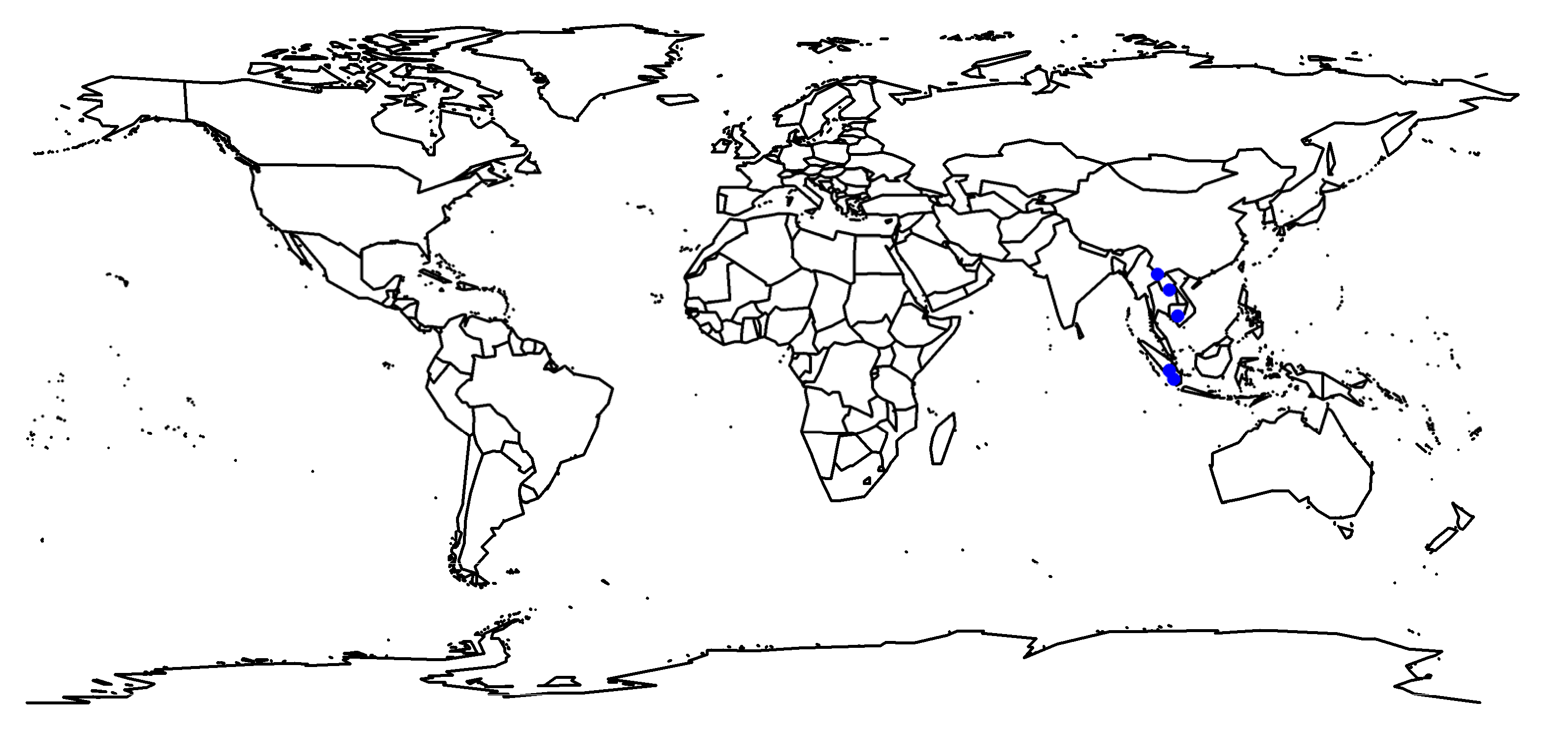
42]. To expand the dataset used for model validation and evaluation beyond the focus area of Jambi province, we additionally extracted available data containing carbon and water-related variables in rubber plantations using following terms: “rubber plantations”, “tropics”, “rubber trees”, “subtropics”, “net ecosystem exchange”, “leaf area index”, “transpiration”, “evapotranspiration”, “specific leaf area”, and “rubber tree growth” from the free web search engines Google Scholar and Web of Science. Selection criteria for data inclusion were matured rubber plantations and field grown rubber trees. A spatial display of all sites used in this study is shown in
Figure A1. We were able to obtain six articles corresponding to up to five different rubber plantation sites. These plantation sites were located in Indonesia, Cambodia, Thailand and China.
2.2. Model Initialization
Similar to many land surface models [
43], CLM needs to be spun up to bring all soil and vegetation carbon and nitrogen pools into equilibrium [
31]. Therefore, to estimate the vegetation and soil biogeochemical state before the establishment of the rubber plantation in Jambi, the model was first spun up to a preindustrial equilibrium state with a Tropical Evergreen forest PFT and continued with a 20th century transient run until 2001, using the standard procedures of CLM spin-ups [
44,
45]. The Tropical Evergreen PFT for the spin-up was used because it was the region’s dominant natural vegetation before the agricultural-driven land-use change. For spin-ups, we used site-level measurements of soil texture [
12], the preindustrial value of CO
2 concentration (284.7 ppm), and recycled the climate data of 1900–1972, extracted for the Jambi lowland from CRUNCEP data [
46] for the duration of the simulations. CRUNCEP uses two types of data: one that is derived using the NCEP reanalysis at a 6 h time step and 2.5 resolution based on a climate model (that only assimilates the temperatures) and the other the monthly Climate Research Unit (CRU TS Version 4.04) climatology at 0.5 resolution.
We performed the first spin-up by running the model for 300 years in the accelerated mode, whereby the decomposition of slower cycling carbon and nitrogen pools is increased for the duration of the spin-up, and the pool sizes are modified accordingly at the end of the spin-up [
28,
31]. Then we ran the model for another 300 years in the normal mode to get to the ecosystem equilibrium state. We performed a transient simulation following spin-ups, where we used the CRUNCEP climate data [
46] and transient CO
2 across years. Since historical data on CO
2 concentration and N deposition were available from 1850, the transient simulations were performed from 1850 until 2000.
Following the spin-up and 20th century simulations, a clear-cut site disturbance was implemented in the year 2001 by setting the aboveground carbon and nitrogen pools to zero. To this end, we transferred the fine root and coarse root carbon and nitrogen into the litter pools. Then a rubber plantation simulation in Jambi was performed from 2001 to 2014 using the site-level half-hourly climate data [
47]. We simulated two separate rubber PFT simulations: (1) one that used baseline parameter values of tropical evergreen PFT and its corresponding functions (hereafter referred to as “AS_EVG”) and (2) the other that used baseline parameter values of tropical deciduous PFT and its corresponding functions (hereafter referred to as “AS_DEC”).
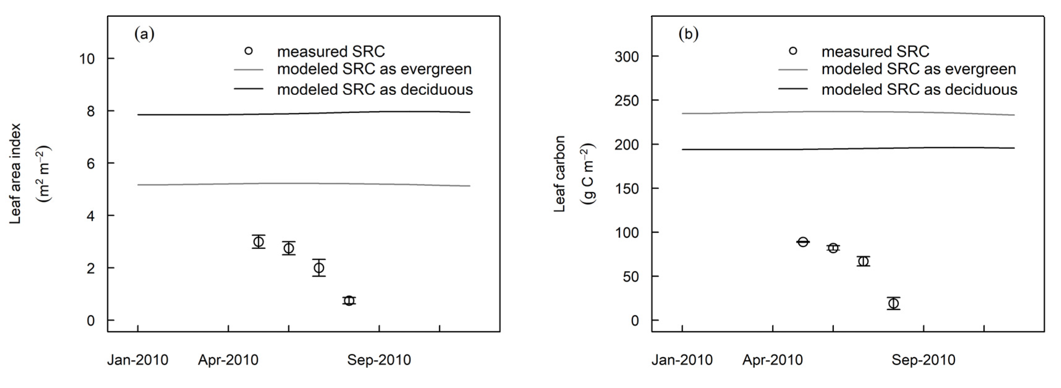
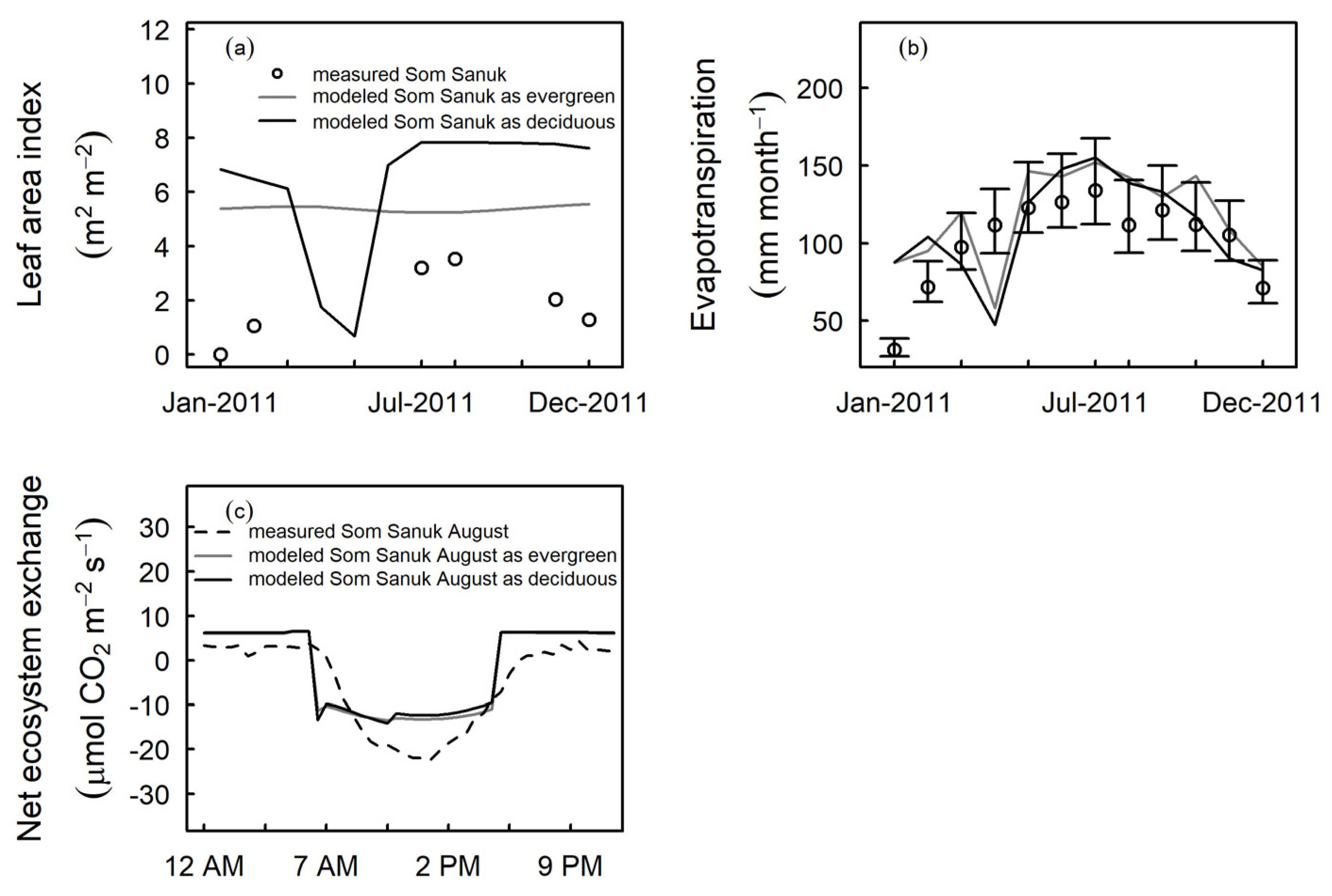
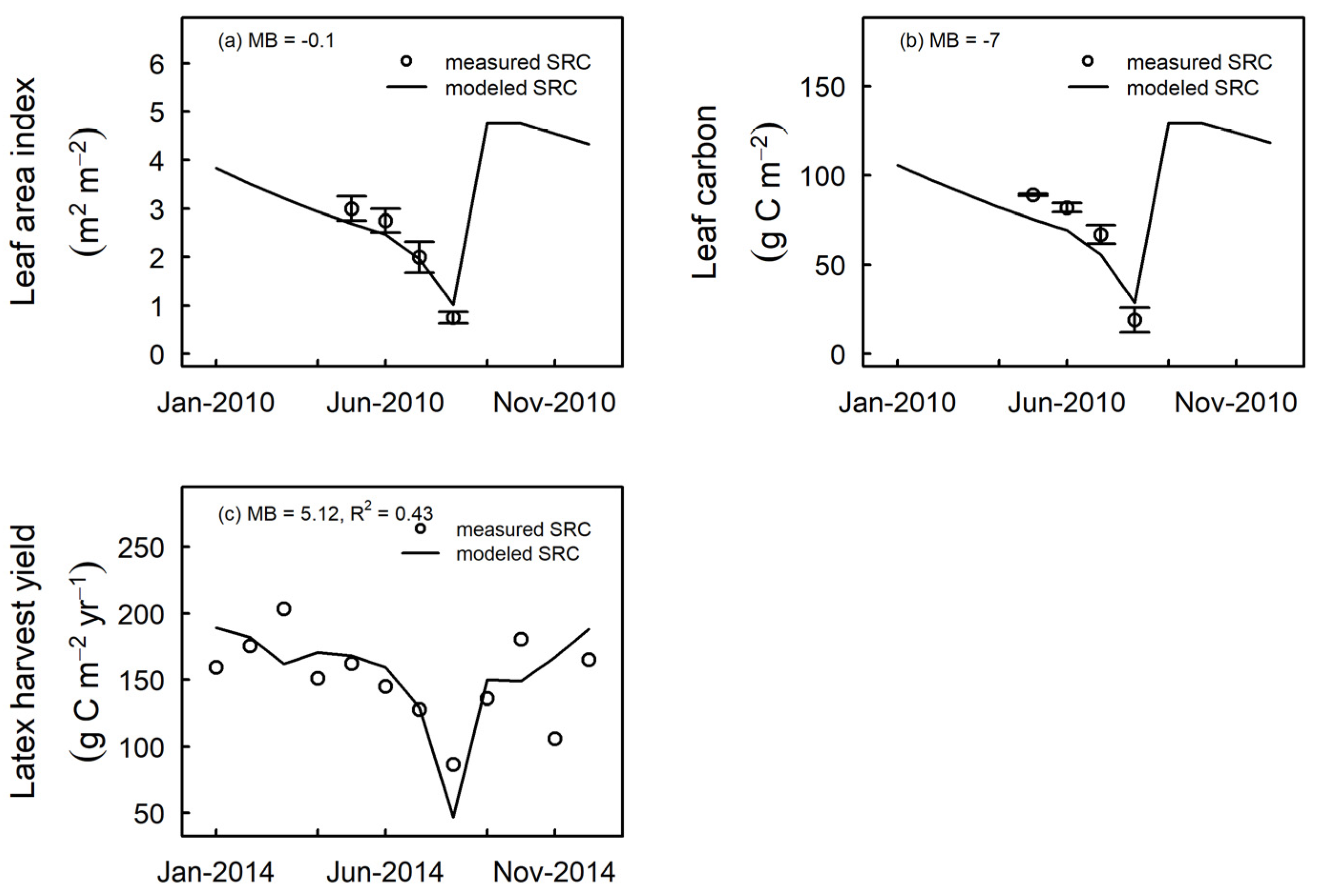
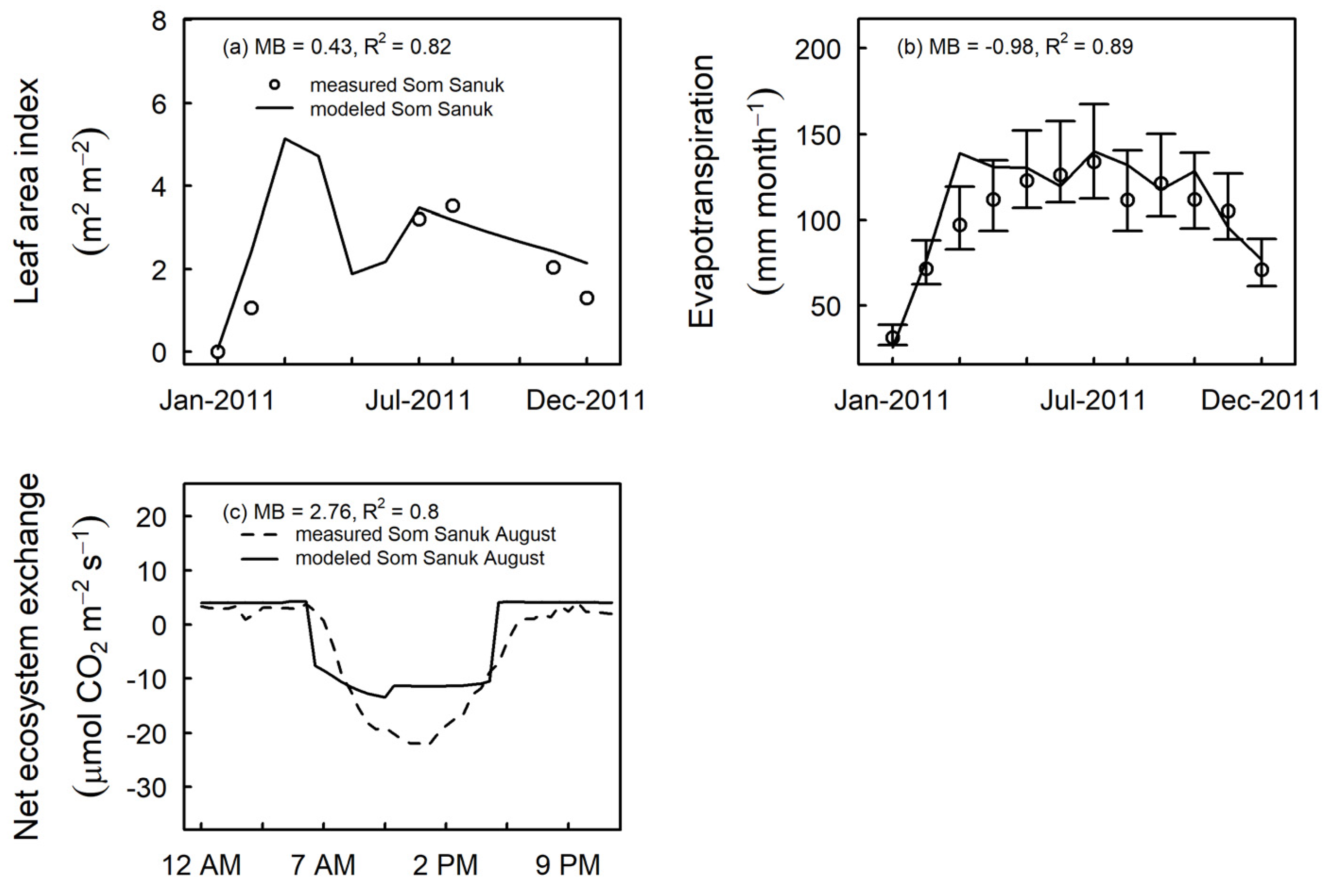
To evaluate rubber PFT simulations at other sites (those that differ in climate and soil texture from Jambi), we first obtained data from three different sites: SRC, Indonesia (4° S, 104° E; 10 m elevation); CRRI, Cambodia (11.6° N, 105° E; 57 m elevation); and Som Sanuk, Thailand (18.1° N, 103° E; 210 m elevation), and then we performed separate simulations at each site for the “AS_EVG” and “AS_DEC” types using each PFT’s baseline parameter values and their corresponding functions. To carry out these rubber PFT simulations at these additional sites, a similar protocol was used as in the case of Jambi, Indonesia. That is, we used their site-specific soil texture and CRUNCEP climate data [
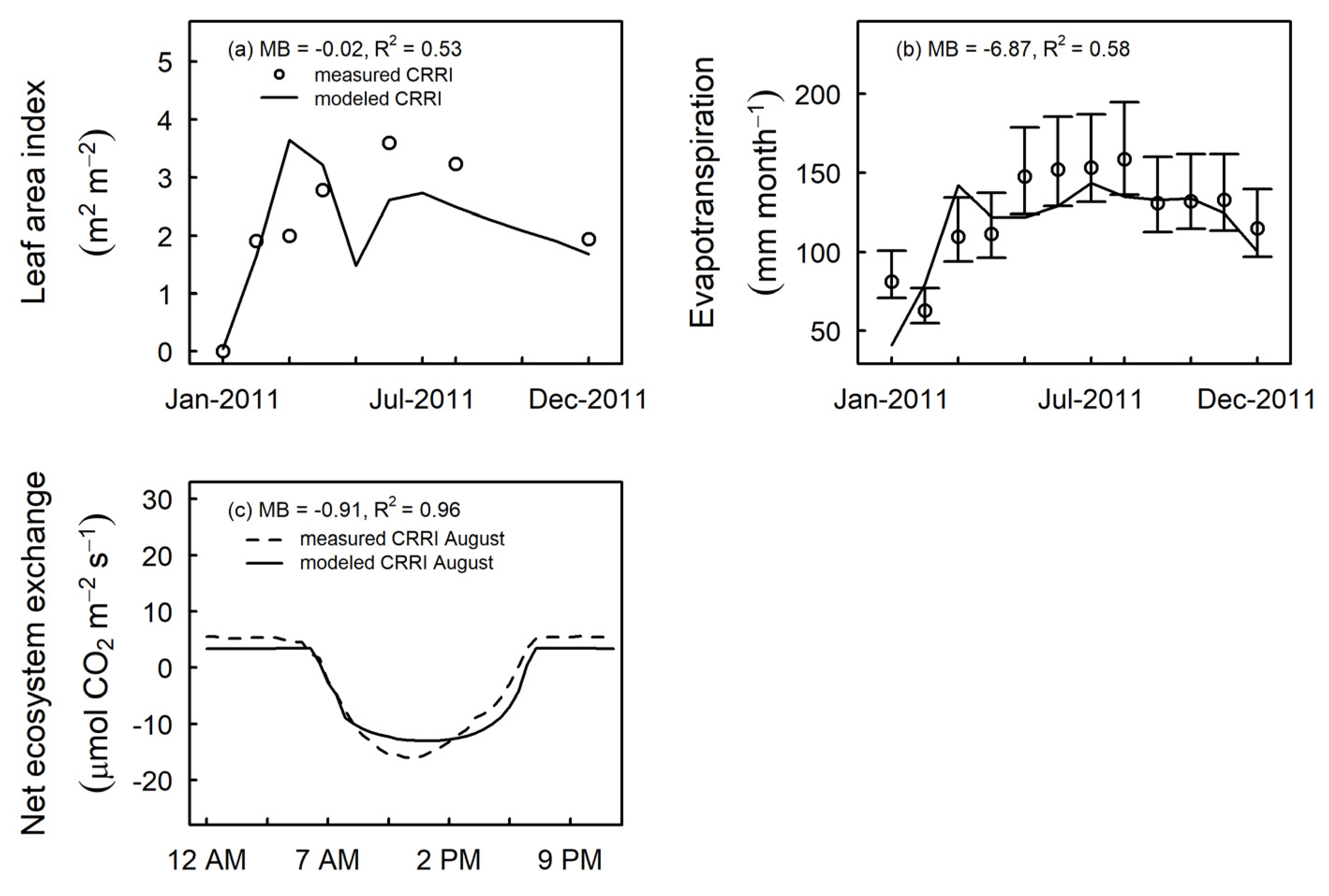
46] to perform spin-ups and transient simulations from the year 1850 up to the year before the clear-cut site disturbance was implemented. At that time point, a clear-cut disturbance at every site was carried out by setting the aboveground carbon and nitrogen pools to zero. As in the case of Jambi, we transferred the fine root carbon and nitrogen into fast litter pools at every site. Next, a rubber plantation simulation was performed at each site from their clear-cut year to year 2014 using the site-level half-hourly climate data. The source of the local climate data follows: the data from SRC were directly available to the authors; for the CRRI and Som Sanuk sites, the data were adapted from the repository specified in Giambelluca et al. [
10].
2.3. Rubber PFT Development
For the development of the rubber PFT within CLM5, our main goal was to represent the growth characteristics of rubber trees and include a realistic representation of carbon exports via latex harvest. We modified the phenology and allocation schemes of the existing broadleaf tropical deciduous tree PFT to represent rubber’s specific leaf onset, litterfall, and harvest export of latex yield that influence carbon and water cycles.
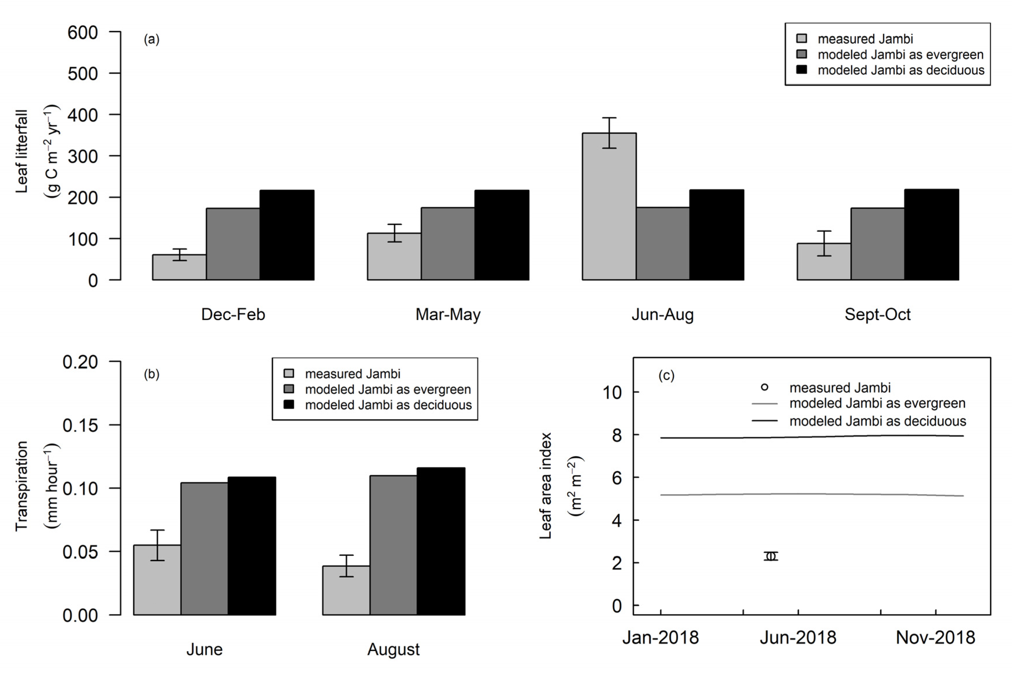
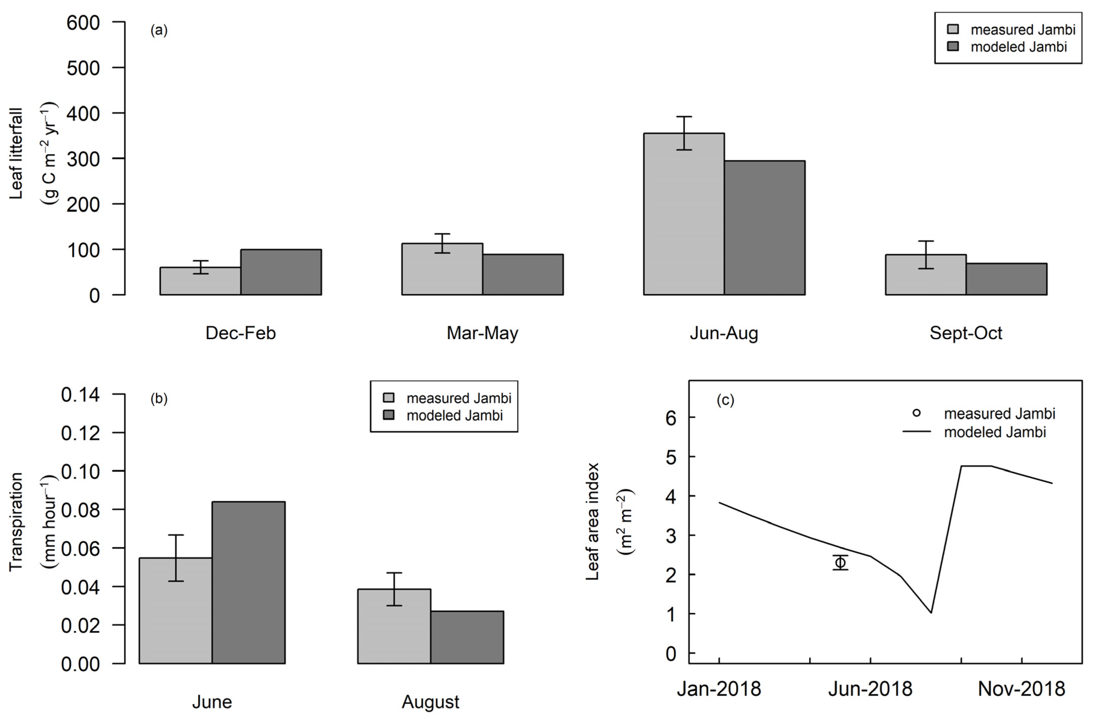
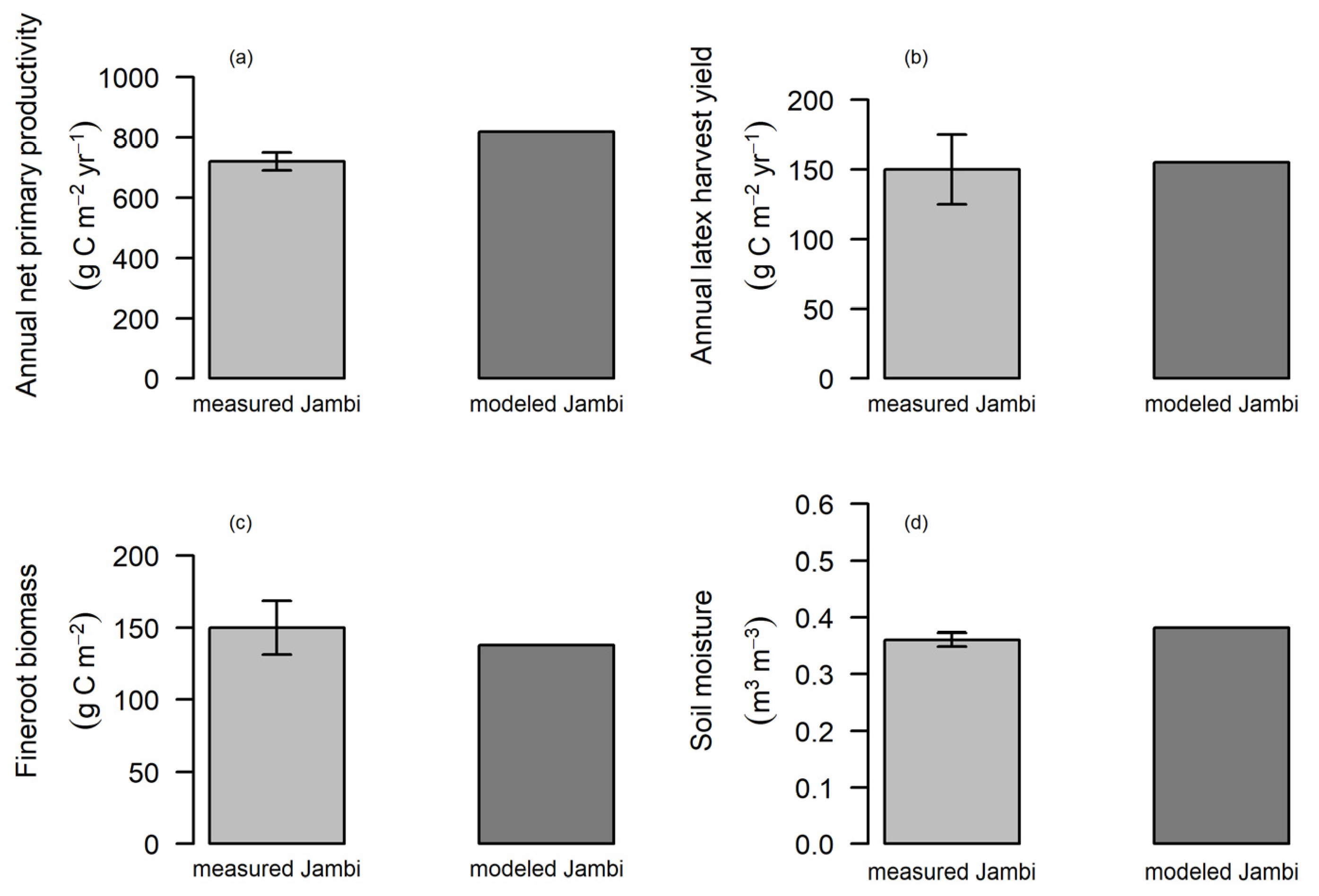
We parameterized and calibrated the model at the Jambi site only. Some parameter values were prescribed using measurement data from Jambi, while other parameter values were obtained via model calibration, e.g., we used measured values of leaf morphological parameters such as the ratio of leaf C to leaf N (leaf CN) and specific leaf area (SLA). For model calibration, we used the specific dataset from Jambi and compared it with Jambi’s model output values. Specifically, these measured Jambi data were leaf litterfall rates, transpiration rates, leaf area index, net primary productivity, latex harvest yield, and fine root biomass. We can consider the final set of parameters (measured and calibrated) for the Jambi model simulation as “optimum parameter set values”. A list of parameters for CLM5 is provided in
Table 1, which shows the default value, measured or calibrated value, and the most affected model output the parameter value impacts (the model is fitted to the corresponding observed values).
2.4. Phenology
We implemented the rubber phenology based on the standard stress deciduous phenology scheme for tropical broadleaf PFT in CLM5 [
31]. We first describe the standard stress deciduous phenology scheme (see
Appendix B and
Appendix C) and then describe our changes in this rubber scheme (see below). The standard stress deciduous phenology scheme in CLM5 [
31] is based on Dahlin et al. [
30] that allows plants to shed their leaves through two different mechanisms: (i) leaf onset/offset—where this switch is triggered by sustained periods of wet or dry soil (
Appendix B); (ii) a background leaf litterfall rate, which is calculated using leaf longevity (
Appendix C). The background leaf litterfall rate is not associated with a specific offset period but occurs over an extended time.
2.5. Phenology Scheme for Rubber
The changes we have made in the standard stress deciduous phenology scheme for rubber are based on the following observations. Foremost, we set the leaf longevity (γ
leaf) of rubber trees to one year because rubber trees exhibit annual shedding of senescent leaves [
50].
Secondly, the defoliation (leaf offset), also referred to as ”wintering”, is usually seen in rubber trees once they are matured, that is, once they are greater than 4 years old [
50,
51,
52]. In the Northern Hemisphere, specifically in mainland Asia (e.g., Cambodia and Thailand), rubber plantations have been observed to be in dormancy (LAI = 0) for about three weeks in January [
11]. The mechanisms for this dormancy are mixed: reduced soil moisture [
11,
53] or low temperatures when soil moisture had already recovered [
7,
54]. In the Southern Hemisphere, dormancy in rubber plantations has been observed in August [
55,
56]. If the soil is relatively wet and temperatures are relatively high throughout the year, then it is challenging for the model to predict leaf offset (i.e., ”predict dormancy”) as observed empirically. Our preliminary modeling analyses indicated that all of the aforementioned triggers were unable to predict the leaf offset as empirically observed. Since Yeang et al. [
36] and Zhai et al. [
37] suggested that decreases in daylength could also trigger leaves to fall in rubber plantations, we used daylength to trigger leaf offset. Below we present a set of four rules for the initiation of leaf offset for varying daylength (hours) values:
where D
max, D
min is the maximum and minimum values of daylength at a given location, respectively, and d
current and d
previous are the current and previous day’s daylength value at a given location, respectively. The four rules in Equation (1) are evaluated by the logic “OR” and the values in Equation (1) are based on manual calibration. As noted above, we segregated daylength values and also constrain them so that they can be applicable at different sites in Southeast Asia. If the leaves were not in the offset period, then they were in the onset period.
Next, we increased
by multiplying it by 1.5 during the period when the leaf offset was initiated. The value of 1.5 was obtained by fitting the modeled leaf litterfall rates in Jambi to measured leaf litterfall rates in Jambi [
34].
Finally, to avoid much longer periods of modeled leaf offset than observed, we modified the value of offset soil water potential threshold as follows:
where
is the previous 10 days of accumulated rainfall and
is the previous 60 days of accumulated rainfall.
2.6. Allocation Scheme for Latex Harvest Yield
As in the case of phenology, we describe the standard carbon allocation scheme used in CLM5 (see
Appendix D). Below we explain our assumptions for rubber to calculate latex harvest yield and also explain how we obtained the parameter value related to tap**. We assume that due to tap**, the total stem allocation would be partitioned to three pools with the following allometry for CLM-rubber,
where f
tap is the proportion of stem allocation partitioned into latex tap** (f
tap = 0.46) and f
d is the allocation for deadwood (f
d = 1 − a
4 − f
tap). We obtained the value of f
tap by fitting the modeled latex harvest yield of Jambi to the measured latex harvest yield of Jambi. Thus, Equations (A10)–(A13) now change to Equations (4)–(9) as follows;
The carbon flux of the latex harvest yield is calculated as follows,
2.7. Tap** Period
We recognized that there was a marked difference between the tap** period for rubber plants located around the equator versus those growing at latitudes greater than 8°. Around the equator, there was no difference in rubber tap** period between the dry and wet seasons (e.g., Jambi or Sembawa)—meaning there was no resting month when no tap** occurred. In tropical regions (latitude 8–20°), where there is a distinctly dry, wet, and cool season, tap** is stopped every year in February, March, and April (dry season), allowing nine months of tap** and three months of resting period [
57,
58]. For tropical regions (latitude > 20°) where there is a distinctly dry, wet, and cool season, and also experiencing hail events [
54], rubber trees are usually tapped from May through November [
38,
48]. We combined the above information and set up the scheme for prescribing the tap** period at the site as follows:
The implication of Equation (10) is that it facilitates changes in carbon allocation patterns of rubber plantations spatially.
2.8. Model Calibration
We did not use a formal optimization method to obtain the parameter values because we lacked data from which we could ascertain ranges for all parameters. Instead, we calibrated the model by looking at different processes one at a time (mostly), which means that for every process, we made some assumptions or had some logic. First, we tried to obtain reasonable phenology (leaf area index dynamics) based on four distinct ranges of latitudes. Second, to avoid more extended periods of leaf offset at latitudes away from the equator, we reduced the default value of critical soil water potential (from −0.8 to −2 MPa). Third, the default leaf longevity was about 0.48 years, which seemed low, so we increased it to 1 year. Fourth, the allocation ratio of stem to leaf from 2.3 is reduced to 1, where we assumed rubber trees allocate carbon similarly in leaves and stems. The second, third, and fourth changes were made simultaneously, and the model was run. Model outputs were compared with measurements.
We increased the multiplier factor (from 1 to 1.5) to increase litterfall rates in the dry season. We ran the model several times here because we changed the value in increments of 0.1 and compared the model values of litterfall against measurements. Ultimately we were able to arrive at the critical value, i.e., 1.5. The other calibrated parameters, ftap, dsladlai, and medlynslope, were jointly calibrated—meaning that we manually adjusted these three parameters together. The direction of change of these parameters was determined by comparing the model and measured values of latex yield and transpiration. The model was then run, and model outputs were compared with measurements. We repeated this process several times until we arrived at their optimum values.
2.9. Rubber PFT Simulations and Evaluations
Using a clear-cut site disturbance implementation for Jambi (see above), a rubber PFT simulation in Jambi was performed for the period 2001 to 2014, where the parameters of the model (optimized parameter values;
Table 1) were obtained either through field measurements or using model calibration methods [
44,
59]. See the rubber PFT development section for specific details about how the “optimized parameter values” of rubber were obtained. To evaluate rubber PFT simulations at other sites (SRC, CRRI, and Som Sanuk) that use the optimum parameter set values (
Table 1), a rubber plantation simulation was performed for each site from their clear-cut year through the year 2014.
In this study, two different metrics were used to quantify model performance against the observed datasets. One is a model bias (MB) and the other is based on goodness-of-fit value (the R
2 value) [
60,
61]. MB was calculated as the mean of the model observation residuals [
62]:
where
and
are the observed and model-simulated values, respectively.
A positive bias indicates that the model overestimated the observation data. The determination of coefficient of the ideal model is close to 1 (R
2 = 1 and MB = 0). If the modeled values yield an R
2 value close to 1, but a large bias, we can conclude that the model captured the dynamics of the processes, but relevant parameter values still need further refinement [
27]. For instances where modeled values yield a bias close to 0 with a low R
2 value, we can conclude that the model does not adequately capture the dynamics of the processes [
27], and in this case, a more realistic mechanism needs to be developed to improve the simulation. We present model evaluation for specific variables at individual sites when observation data are available because not every variable is measured at all the sites.
2.10. Comparing CLM-Rubber Model with Other Models
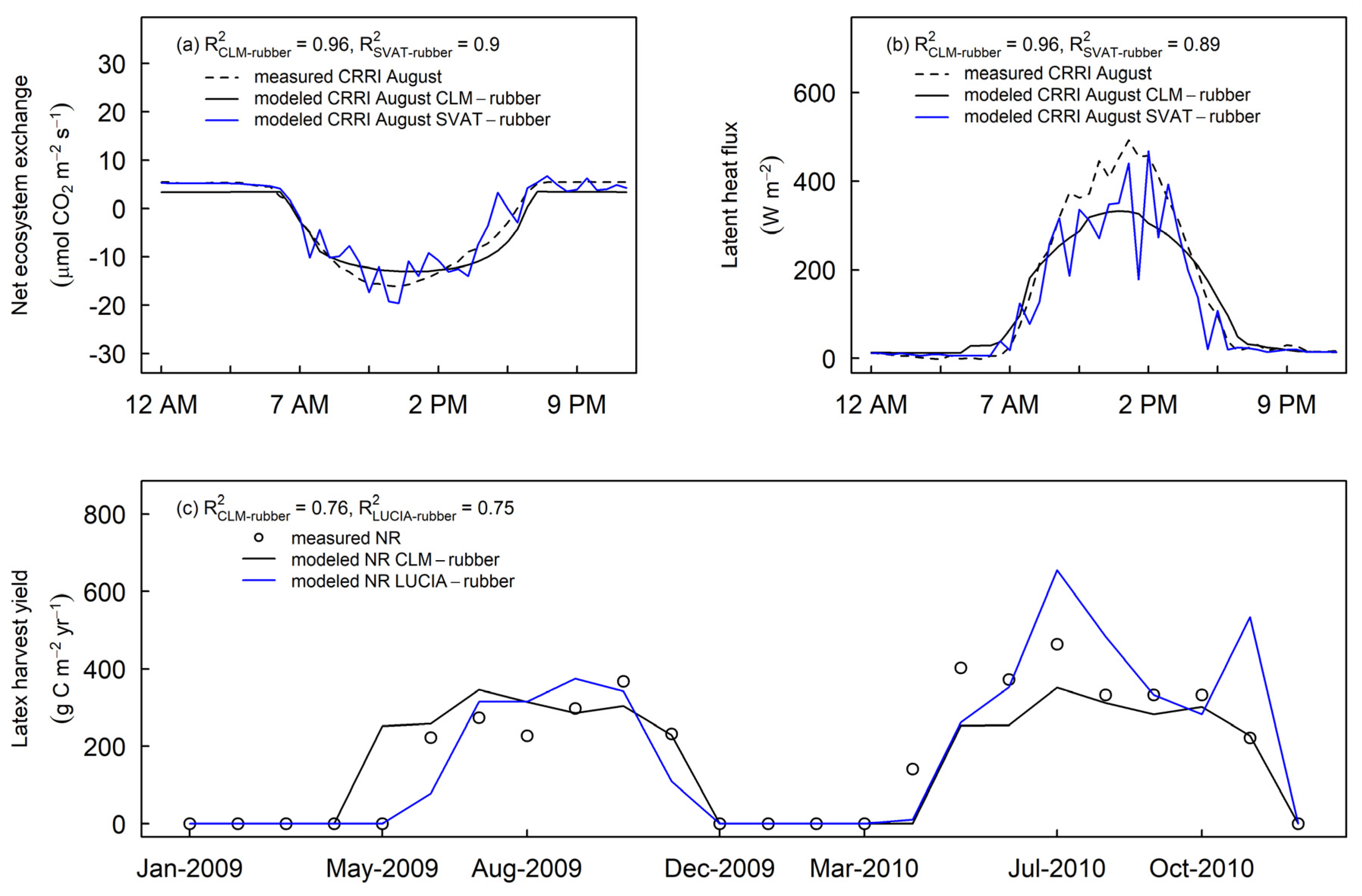
It is important to compare CLM-rubber model results with the existing model simulations from the literature. To this end, we collected data from the literature that performed modeling simulations. We found modeled data on net ecosystem exchange and latent heat flux from CRRI, Cambodia (11.6° N, 103.3° E; 57 m elevation) (SVAT-rubber model; [
15]) and modeled latex harvest yield data from Neban Reserve (NR), China (22° N, 100° E; 680 m elevation) (LUCIA-rubber model; [
16]). We performed CLM-rubber simulations at these two sites by essentially following a similar scheme as mentioned above and compared our results with the SVAT-rubber and LUCIA-rubber models.
4. Discussion
Our modeling efforts aimed to simulate the phenology, allocation, and latex yield of rubber plantations from Southeast Asia using CLM5. We show that the newly developed rubber PFT and related parametrization outperforms the baseline parametrization of tropical evergreen or the baseline tropical deciduous PFTs in CLM5 for simulating the leaf area index, carbon, and water fluxes of rubber plantations. Our modeling work shows that daylength can be used as a universal trigger for defoliation and refoliation of rubber plantations. Our model can predict reasonable seasonal patterns of latex yield despite highly variable tap** periods across Southeast Asia. Finally, we show that CLM-rubber performs similar in simulating carbon and energy fluxes to the existing rubber model simulations available in the literature.
4.1. Tropical Evergreen and Deciduous Simulations
For rubber plantations growing at latitudes lower than 8°, the model that used baseline tropical evergreen or the baseline tropical deciduous functions and parameterization could not predict the seasonality of litterfall because the rate coefficient for background litterfall was invariant over the seasons. The seasonality of LAI and leaf carbon by both forest types models were also not properly simulated at these sites because the modeled soil water was not low enough to trigger the leaf offset. The magnitudes of LAI and leaf carbon were also primarily overestimated. The likely reasons include parameters related to photosynthesis, e.g., stomatal conductance and parameters related to plant growth, such as specific leaf area [
28]. Additionally, how fast specific leaf area changes relative to the change in leaf area index and how much carbon is allocated to different tissues, such as the ratio of stem: leaf [
31], can attribute to overestimation of LAI and leaf carbon.
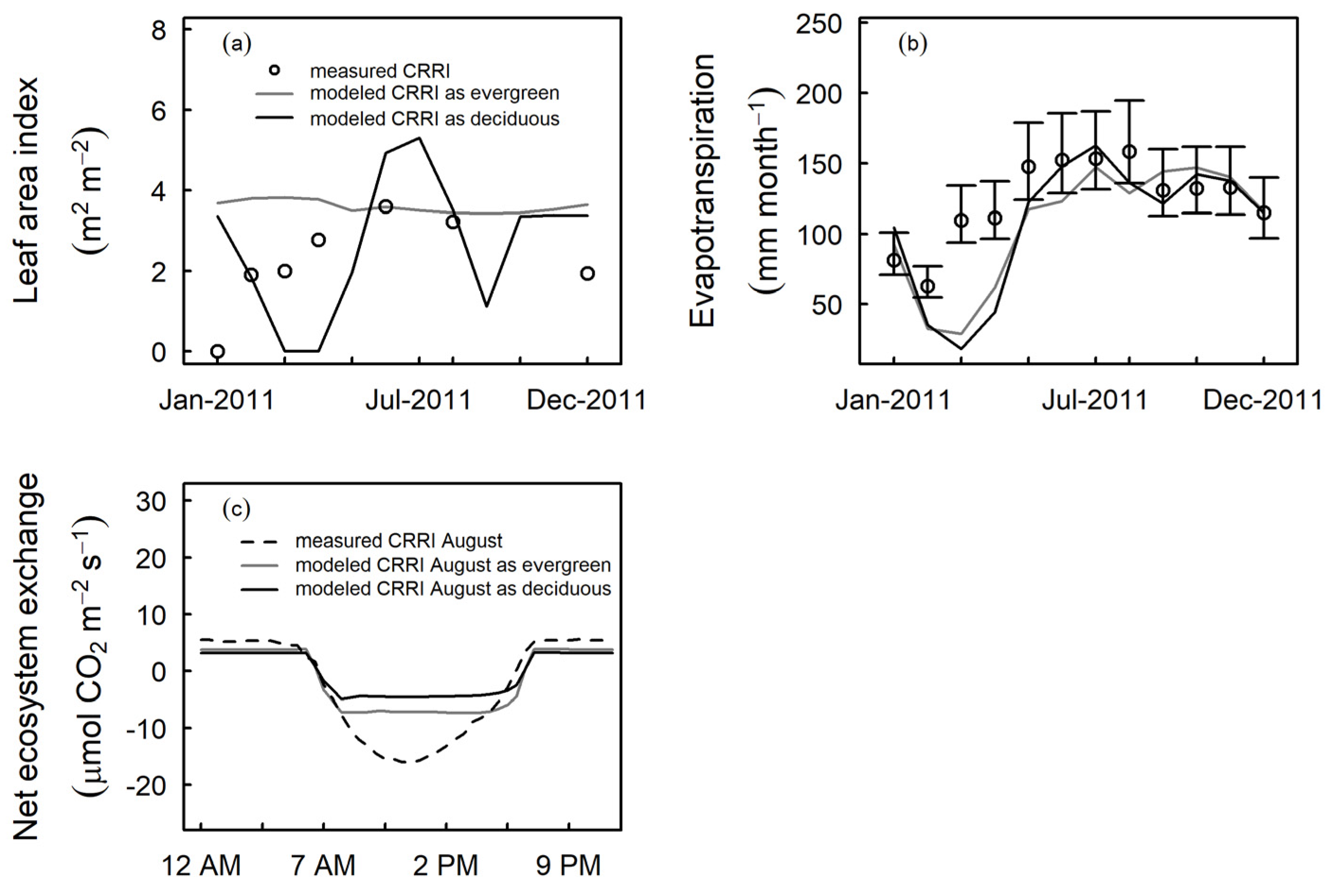
For rubber plantations growing at latitudes greater than 8°, the model that used baseline tropical evergreen or the baseline tropical deciduous functions and parameterization could not predict the proper seasonality of LAI. However, the model that used baseline tropical deciduous functions and parameterizations was better in predicting the seasonal patterns of LAI than the model that used baseline tropical evergreen functions and parameterization. The reason for this discrepancy is that former model was able to trigger leaf offset as the modeled soil water reached low values; however, the timing and the duration of the leaf offset were not accurate. In the growing season, sometimes both models predicted reduced LAI, and this result was due to low irradiance, as rainfall was high during this period in both model simulations.
4.2. Daylength, Carbon, and Water Fluxes
We demonstrated in this study that increasing the background litterfall rate enables modeling of the seasonal cycle of leaf litterfall rates in Jambi, Indonesia. The observed seasonality of leaf litterfall could be controlled by a combination of climatic factors or soil conditions. Our model predicted the peak of the monthly leaf litterfall rate at Neban reserve, China, as February, and this modeled result is in agreement with a rubber plantation in China [
38], where January is typically the coldest month, and leaf shedding occurs after the coldest month [
38]. These results indicate that CLM-rubber will predict reasonably well the seasonality of leaf litterfall of rubber plantations across Southeast Asia.
Our modeling work shows that daylength can be sufficient to represent regional heterogeneity for both the leaf offset and leaf onset of rubber plantations. Daylength works not only for sites with a pronounced dry season [
10], but also for sites in Indonesia where soil moisture may never drop to a critical level. Since rubber plantations are facultative deciduous or semideciduous, we are confident that daylength, as implemented in our study, can be directly used for simulating phenological cycles for other facultative deciduous ecosystems (semideciduous) from Southeast Asia that are managed, such as teak plantations [
66] and cocoa plantations [
67]. Additionally, daylength can also be implemented in CLM5 to potentially improve simulations of unmanaged ecosystems such as semievergreen natural forests in Thailand [
68].
The magnitude of the monthly latex yield simulated by CLM-rubber matched quite well with the observations at the independent sites: the SRC site (Indonesia) and at the Neban reserve site (China). This was an unexpected result because we did not consider tap** frequency in the model. We are aware that tap** frequency generally varies among plantations—two tap** days and one resting day or one tap** day and two resting days [
10]; in the model, we assumed that the proportion of tap** assimilate allocation is constant.
The relatively high R2 values of modeled evapotranspiration rates at the evaluation sites suggest that the model captured the dynamics of processes. Overall, CLM-rubber was able to capture the average trend of carbon and water fluxes of various rubber plantations (R2~0.73, p-value < 0.05), which meets the general purpose for representing a PFT in a land surface scheme.
4.3. Intermodel Comparisons
We compared the simulations of CLM-rubber with simulations of SVAT-rubber and LUCIA-rubber. We also evaluated these models against field observations at the CRRI and Neban sites. CLM-rubber successfully captured the trend of net ecosystem exchange and latent heat flux at the CRRI site because it has the improved seasonal cycle of leaf onset/offset. SVAT-rubber better captured the magnitude of these fluxes (at times) compared to CLM-rubber because it was initialized by prescribing the initial value of LAI as 3.89 m
2 m
−2 [
15], which is almost the peak value of measured LAI for rubber plantations.
CLM-rubber captured the seasonality of latex yield at Neban reserve because CLM-rubber was able to allocate carbon to different tissues properly, and it also predicted the proper leaf shedding period. On the other hand, LUCIA-rubber predicted delayed leaf flushing (shown to be up to a 2 month delay) and subsequently underestimated latex yield [
16]. Our model comparisons indicate that CLM-rubber generally performs similar to the other two models—this highlights that the modeling efforts for rubber in CLM are viable and valuable.


 ,
, 


