1. Introduction
Whenever one deals with a process involving randomness (stochastic process), it is of interest to empirically determine the frequencies of the various occurring events. The ratios of these frequencies divided by the total number of occurrences are named relative frequencies; the frequencies provide an estimation of the probabilities of the events, which, together, compose the distribution of probabilities of the process. George K. Zipf (1902–1950), a Harvard graduate of 1923, determined the frequencies of the words in large collections of texts and found that, after arranging the words , according to their relative frequencies, , from the highest to the lowest, the relative frequencies were approximatively proportional to the inverse of word ranks, , , where was a constant depending on the number of words in the analyzed text. This became known as Zipf’s law, and the probability distribution is known as the Zipf’s distribution. Zipf’s law is a member of a larger family of distributions, frequently named the power low distribution, defined by . Often, especially when a power law is determined for collections of texts, is still referred to as Zipf’s law. It is common to take the logarithm of the relation defining Zipf or power laws, ; this is the equation of a line , where , , and . Zipf went on to find that the populations of the towns and cities in the US also obey a power law. Zipf, who had a professorship at Harvard until his death, tried to construct an explanation (i.e., generative model) for this specific distribution occurring in many social processes, including language. One of his last works, “relative frequency and dynamic equilibrium in phonology and morphology”, presented in 1949 at a conference in Paris, France, was devoted to the subject. However, we still do not have a convincing model that explains Zipf’s law in linguistics. The purpose of this study is to reveal and explain some elementary properties of Zipf’s law.
There are innumerable papers on Zipf’s law dealing with theoretical aspects and applications. We analyze some elementary consequences of the power law (Zipf’s distribution) in the context of populations that typically satisfy the condition that the elements of the population have a feature expressed by a natural number, and thus they can be ranked. Examples include the set of cities in a country, where the feature is the number of people living in the city, a set of papers, with the feature defined by the number of citations, and the set of words (or lemmas) in a text, with the feature expressed by the number of apparitions of the word. A minor difficulty is that two elements in a set may have equal values of the feature, for example, two words may have the same number of occurrences. This is formally solved by randomly assigning successive ranks to those elements; alternatively, one can assign fractional ranks, but this is a departure from the intuitive concept of rank.
3. Zipf’s Law over Finite Multisets—Properties
When applying Zipf’s law to texts or other similar applications, we have to observe specific properties of the investigated objects. While this is problematic from a linguistic point of view, considering that Zipf’s law is equally valid for lemmas and words, for brevity, we use the term “word” to designate either a word or its lemma. The discussion uses the strong assumption that word occurrences are independent. Also, we assume that:
- (i).
the objects in the population belong to a discrete, finite multiset of prototypes (individual words or lemmas), with the number of replications of the same type of object (multiplicity) not limited in the population; the set of prototypes is denoted by and the ordinal by ; we assume is the vocabulary of a language, or at least a large part of it;
- (ii).
the ordinal of the set of prototypes is much smaller than the number of elements in the population (text); .
In the context of natural language processing (NLP), the set of prototypes is the set of words or lemmas of the vocabulary of a language, the objects are words (or lemmas), denoted by , and the population typically represents a large corpus (a text, in general terms). The situation described corresponds to the case of “Big Data” (vocabularies of tens or hundreds of thousands of words), but the content of this article may also be applied to a small population, such as a novel; in the last case, the vocabulary is specific to the author or is specific to that novel. Even in these particular cases, the vocabulary is much smaller than the population; therefore, the discussion in this article still applies.
Because of (ii), at least some words are repeated a number of times. We denote by the multiplicity of the prototype (word) . The numbers of occurrences of some words may be equal . The fact that is a departure from the “pure” Zipf’s law; some of its consequences are described below.
The property of
combined with
leads to an integer close to
[
5,
25], which may be
, or
, or
, where the symbols [ ], ⌊ ⌋, and ⌈ ⌉ represent the integer part, floor, and ceiling functions, respectively. The choice from the three variants is somewhat arbitrary, but we are sure that, on average,
. This is valid when we do not account for any randomness. The expression “on average” means that, over a large number of texts (corpora) with the same distribution of words, the expected frequency of the word is at least
. The difference between the values
and
can be seen as the equivalent of a noise with two values,
,
.
The constant
is derived from the following condition:
where
is the total number of words in the text,
is the maximal rank, and
is the generalized harmonic number,
, with
;
denotes the Riemann zeta function. Therefore:
Because the multiplicity of any word in a text is either 0 or a natural number, the above has to be corrected, for the application discussed, as:
This establishes a condition for the maximal rank,
:
Therefore, when
and
are known,
is uniquely determined, as intuitively expected. This helps us to estimate one parameter of a text,
, when its size
is known and the standard Zipf’s law (
) is assumed. Considerable departures from the theoretical value of
empirically found signal that standard Zipf’s law is not a good model for the text. For
:
where
is the harmonic number. According to Taeisinger’s result cited by Sanna [
26],
for
; therefore,
for any
; therefore, we were compelled to use approximations for finding
. For large enough
values, i.e., for large texts (corpora) with at least tens of thousands of words:
Above,
is the Euler–Mascheroni constant,
Then:
which solved by approximation methods, provides the estimation of
. For
, one can use approximations of
for determining an approximate value of
. For
and
,
has a known formula; for several fractional values of
, the approximations of
in terms of
are well known, allowing us to efficiently find
for texts of specified sizes.
The finite vocabulary
leads to the repetitions of all words in a text when the text is large enough. The minimal text size that guarantees that all the words are repeated is given by:
The multiplicity of an element (word) is a natural number and the finite nature of
is the specific aspect of the end part of the graph of Zipf’s law. This property is well known [
5]; the end part of the graph was named “broom-like tail” [
25] because of the shape similarity. (The results made public by HNT as [
25] have been derived before the author became aware of the book [
5], a reference that is much less cited than it deserves.) First, notice that there may be a rank, denoted by
such that
, due to the equality of the predicted number of multiplicities when forcing to natural numbers the number of elements for a specified couple of successive ranks:
Denoted by
, the smallest rank where multiplicity (i.e., count at least 2) occurs, the above is equivalent to:
The ranks are successive natural numbers,
; therefore:
The equality of the values of the floor function of the two successive elements implies that:
or:
When
, this condition leads to:
which is easy to solve. For a multiplicity of order,
, the condition is:
Consequently,
and, for
, a simple condition easy to solve either in terms of
or
is:
As can be expected, the multiplicity increases with the rank (see
Figure 1). The above discussion allows us to clarify how the tail of the Zipf’s law graph splits and shows a “broom-like” shape; in addition, the discussion shows that this specific shape of the tail is not due to some statistical noise, as suggested by [
27] (“
the statistical noise, … is always present, but is most obvious in the tails of discrete power law distributions”).
Determining the multiplicities for the highest ranks is significant in linguistics, especially in stylometry, where the number of hapaxes in a text are typically determined and may help differentiate authors when texts of similar sizes are compared.
It may be interesting to determine for a text of
words the total number of ranks
, with equal counts (multiplicities). Denote by
the number of ranks with the same multiplicity (count)
; then:
Next, determine the maximal and minimal ranks that have the same count
:
Then,
. Notice that
depend on
and on
; thus, a more appropriate notation is
. We were interested in the distribution of
. Based on the simulations (see
Figure 2a,b), we conjectured that the distribution was a power law with the power depending on
. Simulations such as those presented in
Figure 2 may help predict the number of expected hapaxes and dis- and tris-legomena in a text and determine if, from this point of view, the text style corresponds to power law distribution of the words.
4. Power Laws with Variable or Noisy Exponents
Empirical data often produce graphs that differ from a typical Zipf one. As previously mentioned, several variants of the power law were proposed for explaining the data, including Mandelbrot and lognormal distributions. However, a good formal approximation of the empirical data is not enough if one cannot find a theoretical (generative) model that explains the distribution production by the application at hand [
28,
29]. In addition, one should validate the matching of the data to the specific distribution used to model them, but distribution tests are seldom reported. Many distributions can produce graphs that apparently resemble Zipf, Mandelbrot, or lognormal laws, where the second part of the graph, for large ranks, seems to be a line with a slope unlike that of the part of the graph. When the second part of the graph is slightly different from a line, one may need to find a better matching distribution. For example, a family of distributions of probabilities
, with variable power, where the power depends on the rank,
has graphs, such as those in
Figure 3. These distributions are candidates for modeling data when the second part of the graph is not a line.
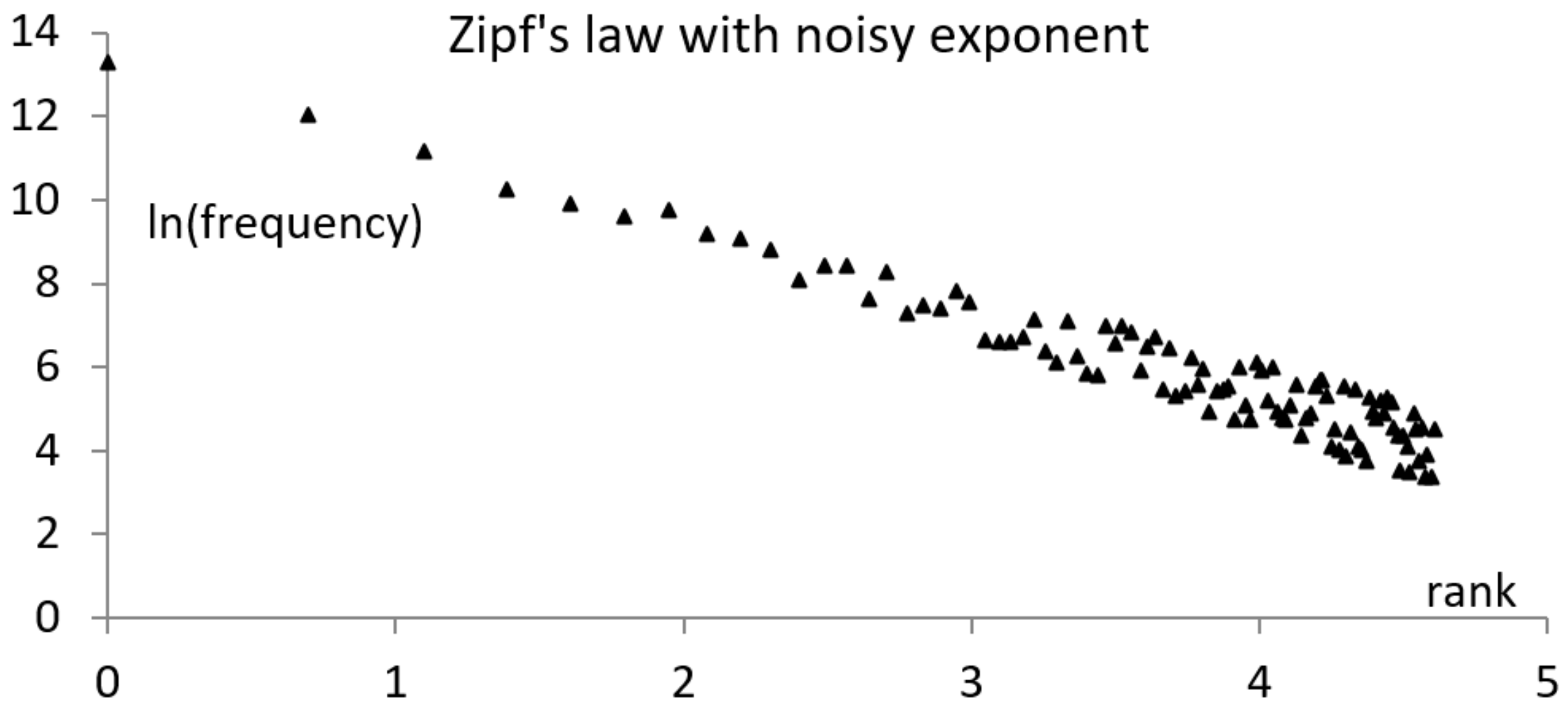
While the noise is not required for explaining the staircase aspect of the end of the graph for Zipf’s law, as already mentioned, noise can affect the data, making it difficult to find the power, of the power distribution. The typical solution is to consider an additive noise, , and to determine the best line matching the data. However, this procedure does not explain heteroscedasticity as, sometimes, it is observed and manifested by an increase in the variance with .
In cases of corpora that include different oeuvres of an author, one frequently finds that a specific word changes the rank, depending on the texts in the corpus. This can be interpreted as an uncertain rank,
, or as an uncertain power. The last interpretation leads to the model
, which exhibits heteroscedasticity (see
Figure 4).
In the next two sections, we applied the properties mentioned above determined for empirical cases.
5. Mixtures of Populations with Power Laws and Etymological Populations
We discussed the case of populations exhibiting a low power distribution and that consisted of subpopulations that also followed a power law. The topic is important in linguistics when one studies a text where the words fall into several categories, for example, neologisms, common words, and archaisms, or words of various etymologies. Another case is that of collections of texts where some of the texts carry negative sentiments, positive sentiments, or are sentiment neutral. We were not aware of any similar applicative treatment, but the main ideas originated from a similar analysis [
30] applied to multinational companies and their subsidiaries [
31].
Assume a population
, with the rank-frequency law according to Zipf,
, and a partition into two sub-populations (sub-multisets),
,
. Furthermore, assuming that
also follows Zipf’s law,
, where
represents the ranks in
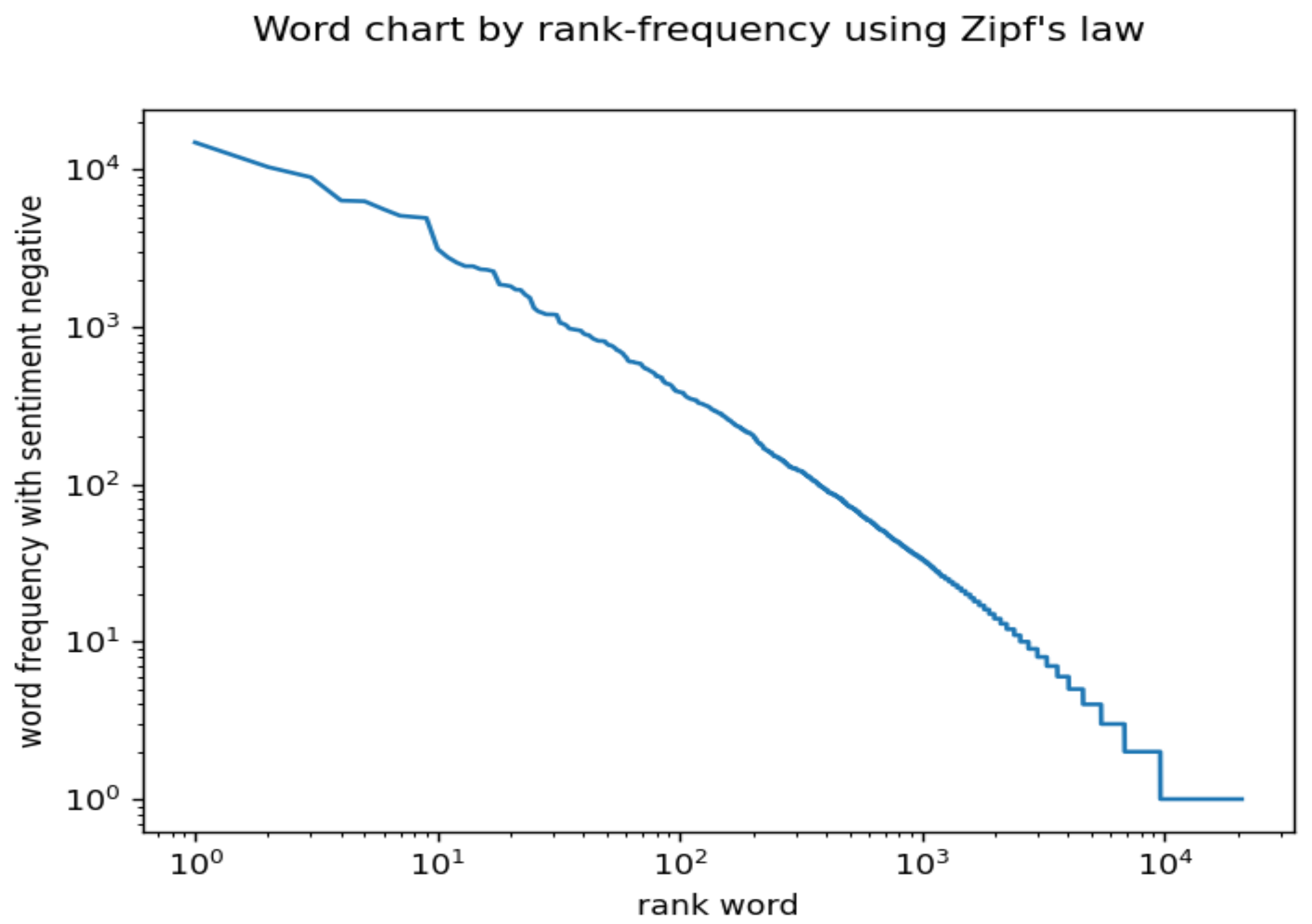
, we are interested in the consequences of this situation where a multiset and a subset of it obey Zipf’s law. An empirical example is a large collection of tweets and the subset of tweets that feature negative sentiments and follow Zipf’s distribution, as shown by [
32].
Assume that is the lowest rank of an element from and ; then, for some and values, ; , , etc. Then, , , , etc., showing that, given that has a Zipf distribution, also has a Zipf’s distribution, only by selecting the elements of with ranks as natural multiples of . When is not a natural number, it has to be rounded up, for the rank remains an integer; but, we skipped this detail. Assume that , that is, the subpopulation is a small part of the initial population, and denoting , satisfies the conditions , . Using this approximation, the elements of the subpopulation have the frequencies of .
We are still left with an unknown number of elements in the subpopulation, which is:
where
,
. The subpopulation is small compared with the population when
, which requires that
, the index where the subpopulation starts, is large.
We name “perfect population” a multiset
, which is a finite union of finite, disjointed multisets, each of them including a single type of object, with the number of elements in the subsets
satisfying the condition
for all
. As the union includes a finite number of finite multisets, the perfect population
is finite. Because
should be divisible by all integers
from 1 to
; therefore, necessarily,
where LCM denotes the least common multiple and
is an integer. In particular,
The multiset is a model of an ideal Zipf population restricted to a finite set of ranks, with a finite number of elements for each rank.
Consider a subset of a perfect population, as above, is composed of all the subsets: , , , , . Denote , , etc. Then, , , etc. Therefore, is also a perfect population. This shows that a Zipf’s distribution restricted to a finite set of objects does include at least one subpopulation that has a finite Zipf’s distribution. In fact, we can choose any to build such a Zipf subset. The next question is if one can build two perfect subpopulations of a perfect population that are disjointed. The answer is affirmative: one needs to choose two prime numbers, , such that . The last condition is required by the condition that no common multiple index is present; if true, the two subpopulations are disjointed. The condition indicates that the two prime numbers should be large enough. There are several unanswered questions, including the following: Considering a perfect population , and a minimal number of ranks in every subpopulation, what is the maximal number of disjointed perfect subpopulations? It is clear that we can construct several disjointed subpopulations—possibly with a single rank—at least equal to the number of prime numbers between and .
The implications of the above presentation are discussed in the next section.
6. Applications, Discussion, and Conclusions
In relation with social networks, particularly Twitter (currently X), Zipf’s law has been used to find suspicious patterns of communication [
33] and for sentiment analysis [
32]. Suggestions that words follow Zipf’s law, when words are used on social networks for subjects related to various events, have been made in studies such as [
34,
35,
36,
37]. We provide an example in
Figure 5, which shows Zipf’s law in tweets with negative sentiment, where the tweets refer to the energy crisis in Europe in 2021–2022. Full explanations are given in [
38]. The example in
Figure 5 parallels the results obtained by [
32].
As large collections of messages on social media exhibit Zipf’s law, the fact that subcollections of messages related to specific events also exhibit an approximate power law requires an explanation. In the same direction, the fact that subcollections of messages that are selected in the criterion of exhibited sentiment may be surprising. The above discussion explains why one can find subpopulations that have a distribution close to Zipf’s one. However, the population,
is no longer a Zipf’s population; yet, when
is small enough, the
distribution can reasonably be approximated to Zipf’s law, as in [
36] and [
32]. Yet, for the data collection presented in [
38], the words related to positive or neutral sentiment have a much greater deviation from a straight line than the negative words.
An interesting partition of a text is obtained when considering the subsets of words with different etymologies. We have analyzed (in [
39] and in the work reported here) several texts in Romanian, also applying the etymological criterion. The etymological analysis method is described in
Appendix A. Similar to English, which has words from Latin, Old German, Old Norse, French, and others, the Romanian language includes words from Latin, French, Old Slavic, Old Greek, Turkish, Hungarian, etc. There is no linguistically known reason to us why the distribution of words with a specific etymology should obey Zipf’s law. Yet, we found that words with certain etymologies followed Zipf’s law closely enough.
Figure 6 presents the segment of the graph for larger ranks for words from Old Slavic; the power of the best line fit was −1.071, and the match to the line was almost perfect (R
2 = 0.99). As is well known, the first part of the graph has a typically less good fit to a line; this occurs also for the data partly presented in
Figure 6. In conclusion, this study clarified some of the properties of Zipf’s law and presented several new aspects of Zipf’s law that pertained to the number theory and set theory.
While the explanation of the possibility of Zipf’s law in subsets of a multiset exhibiting Zipf’s law was proved and discussed in
Section 4, the language mechanisms explaining this surprising behavior remain to be provided by linguists. Extensions to Mandelbrot–Zipf’s and Benford’s laws [
40] could be a natural way to further this study. We can conclude that the analysis of Zipf’s and similar power laws are still a productive field of research, with interesting consequences to be unveiled. Although no explanation exists for why certain phenomena obey Zipf’s law, notable attempts have been made, for example, by Gabaix [
1]; yet, efforts should continue in the future, because few extant explanations are satisfactory, if at all.


