The Modified Helmholtz Equation on a Regular Hexagon—The Symmetric Dirichlet Problem

Abstract
:1. Introduction
- (1)
- a global relation, which is an algebraic equation that involves certain transforms of all (known and unknown) boundary values.
- (2)
- an integral representation of the solution, which involves transforms of all boundary values.
- Given a PDE, define its formal adjoint and construct a one parameter family of solutions of this equation.
- By employing the given PDE and its adjoint, obtain a one parameter family of equations in conservation form. This family, together with Green’s theorem, yield the global relation.
- The above family also gives rise to a certain closed differential form. The spectral analysis of this form gives rise to a scalar Riemann–Hilbert problem, which consequently yields an integral representation of the solution. This representation involves integral transforms of all the boundary values, and since some of them are not prescribed as boundary conditions, this form of solution is not yet effective.
- The explicit solution of the problem is derived by determining the contribution of the unknown boundary values to the integral representation. This can be achieved by using the global relation, as well as equations obtained from the global relation through certain invariant transformations.
Organisation of the Paper
2. The Basic Elements
2.1. The Global Relation and the Integral Representation of the Solution in the Interior of a Convex Polygon
2.2. The Dirichlet Problem on a Regular Hexagon
2.3. The Symmetric Dirichlet Problem
- The modified Helmholtz operator is invariant under the transformation , namely under rotation of . Since the Dirichlet data are invariant under this rotation, then the (unique) solution of the Helmholtz equation is also invariant under this rotation.
- If q is invariant under this transformation, then the differential form is also invariant under the transformation :
- Evaluating the above differential form on each side we obtainwhere the second equality is a direct consequence of the fact that the Dirichlet data are invariant under this rotation.
- (i)
- the odd case, ;
- (ii)
- the even case .
- (i)
- in the odd case, , which yields ;
- (ii)
- in the even case, , which yields for all .
3. Derivation of the Solution for the Symmetric Odd Case
- The zeros of occur when , thus .
- The function is bounded and analytic for .Indeed, if , then . Thus, if , it follows that . Hence, .Therefore, the exponentials and are bounded.
- The function is bounded and analytic for , namely in the region where .Indeed, this expression involves the exponentials and , which are bounded in this region, since .
- The functionis bounded and analytic for .Indeed, since k is at the lower half plane, thenwhich is bounded if .If , then , which yields .
- The function is bounded and analytic for .
- The function is bounded and analytic for , namely in the region where .
- In the lower half planeThus, it is bounded and analytic for .
- 1.
- the fraction remains invariant;
- 2.
- the rays become ;
- 3.
- the exponent becomes ;
- 4.
- the remaining integrands are equal to the corresponding integrands in and .
4. The Symmetric Even Case
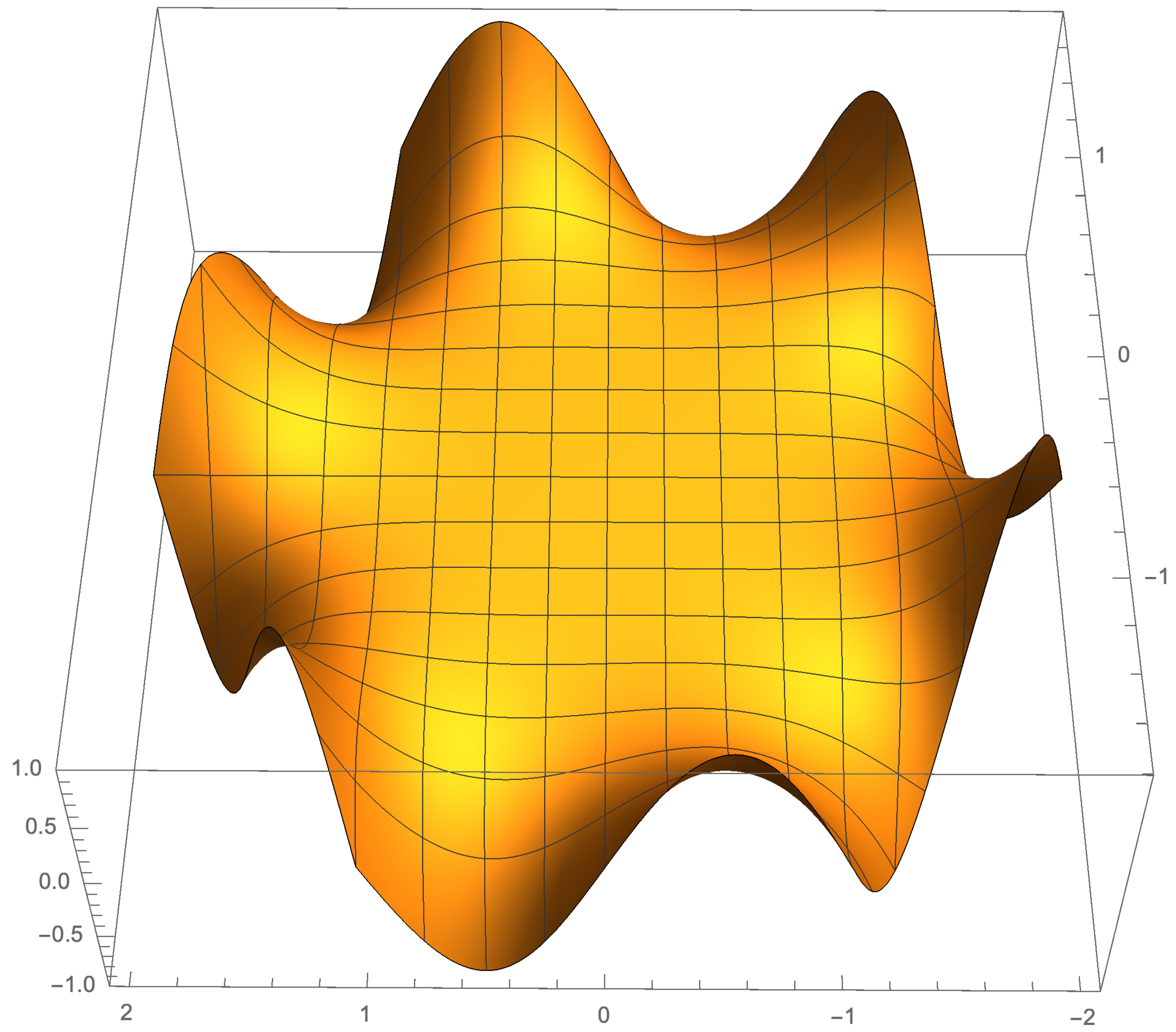
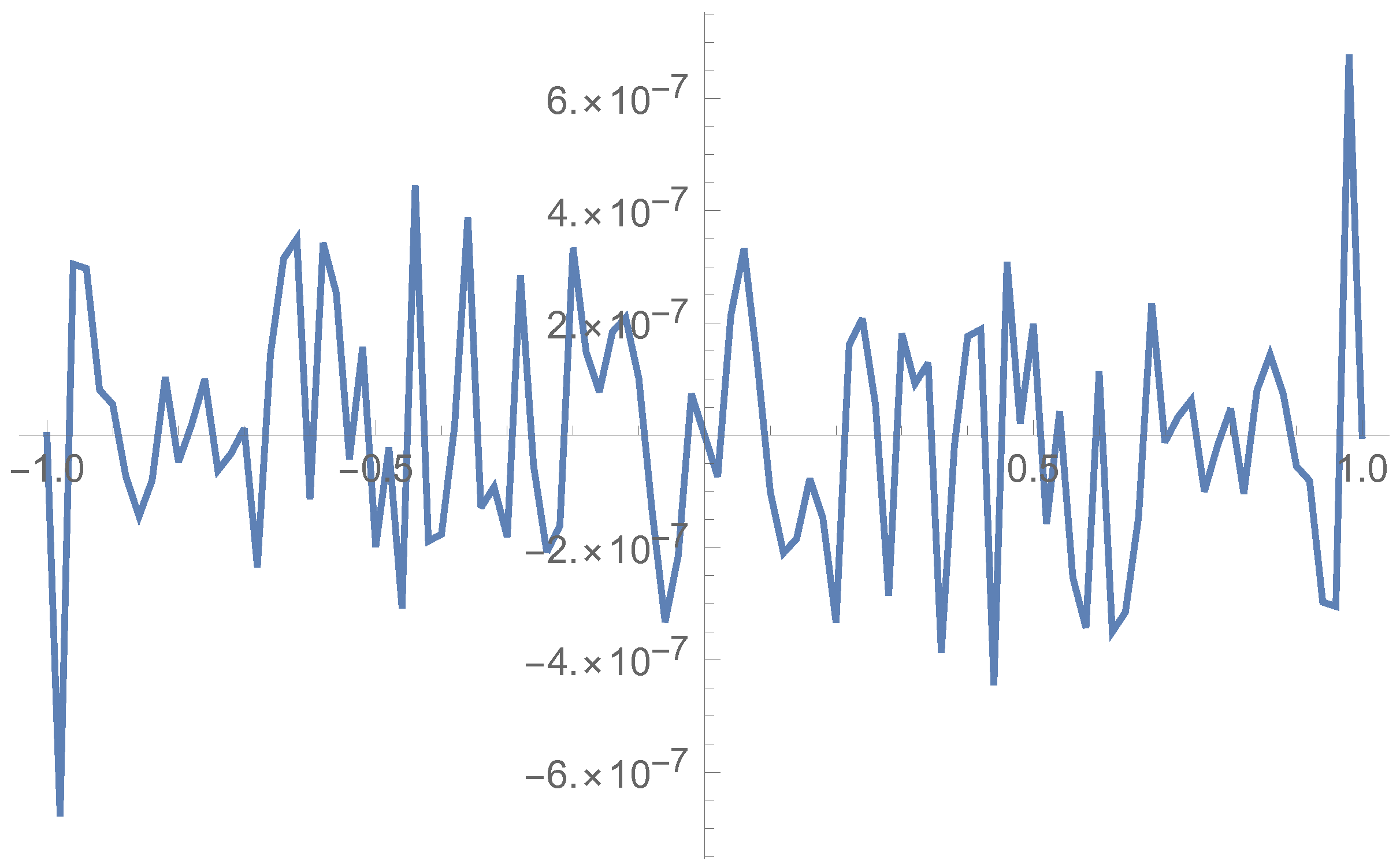
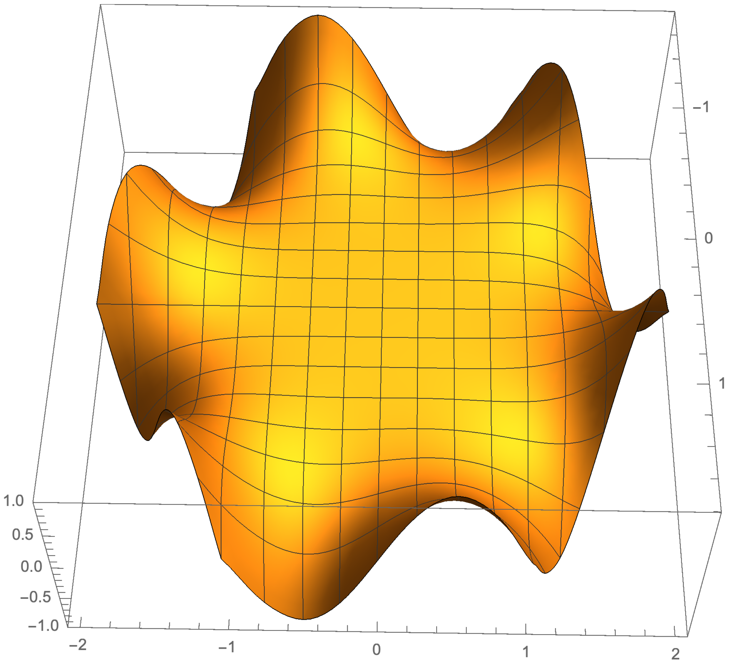
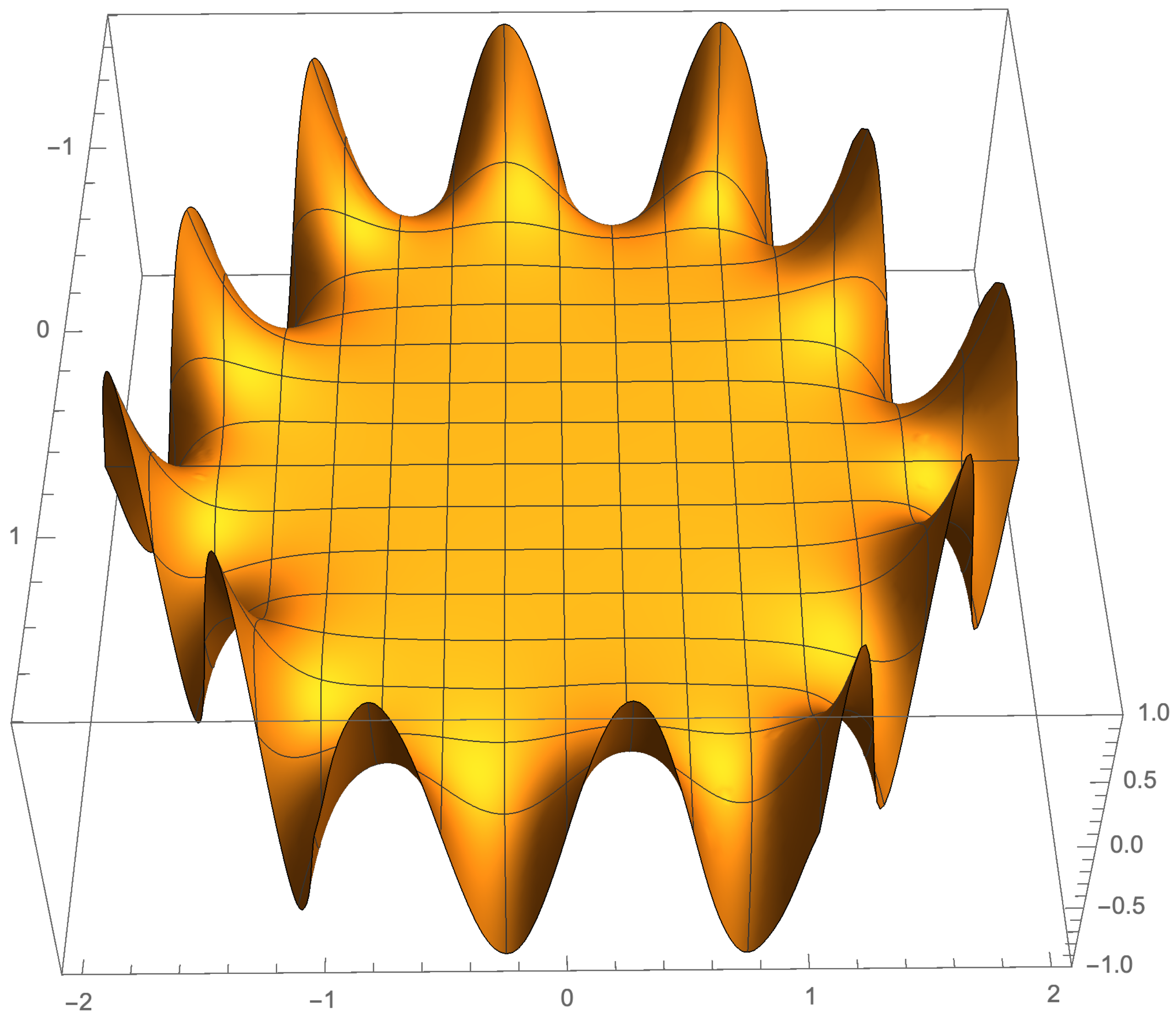
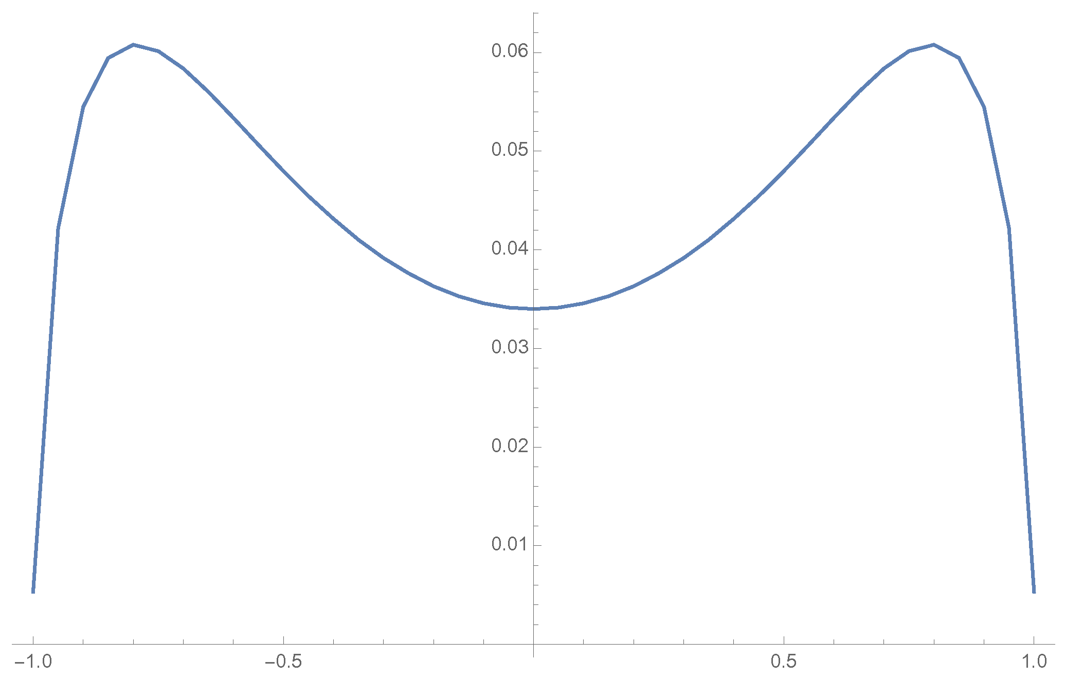
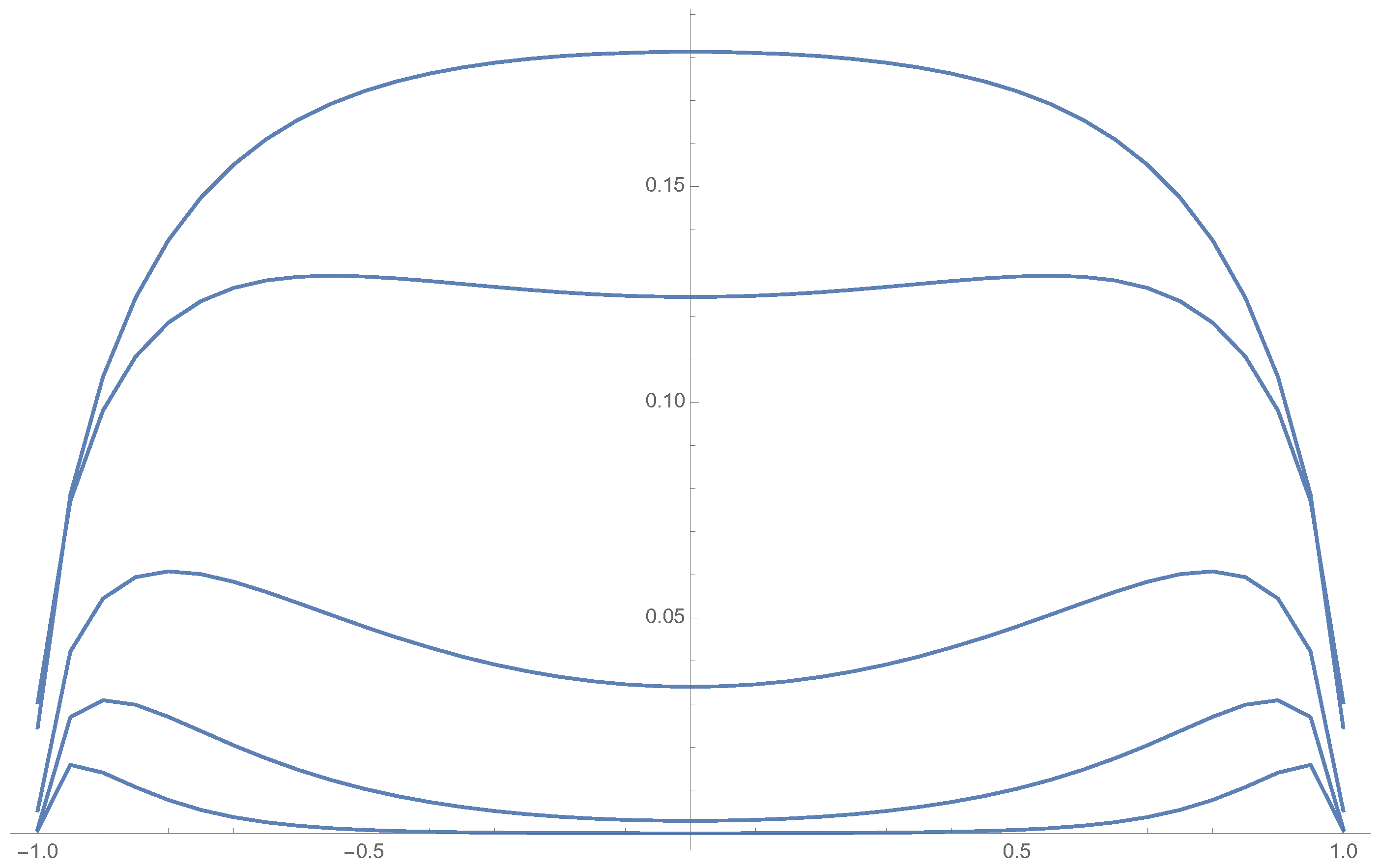
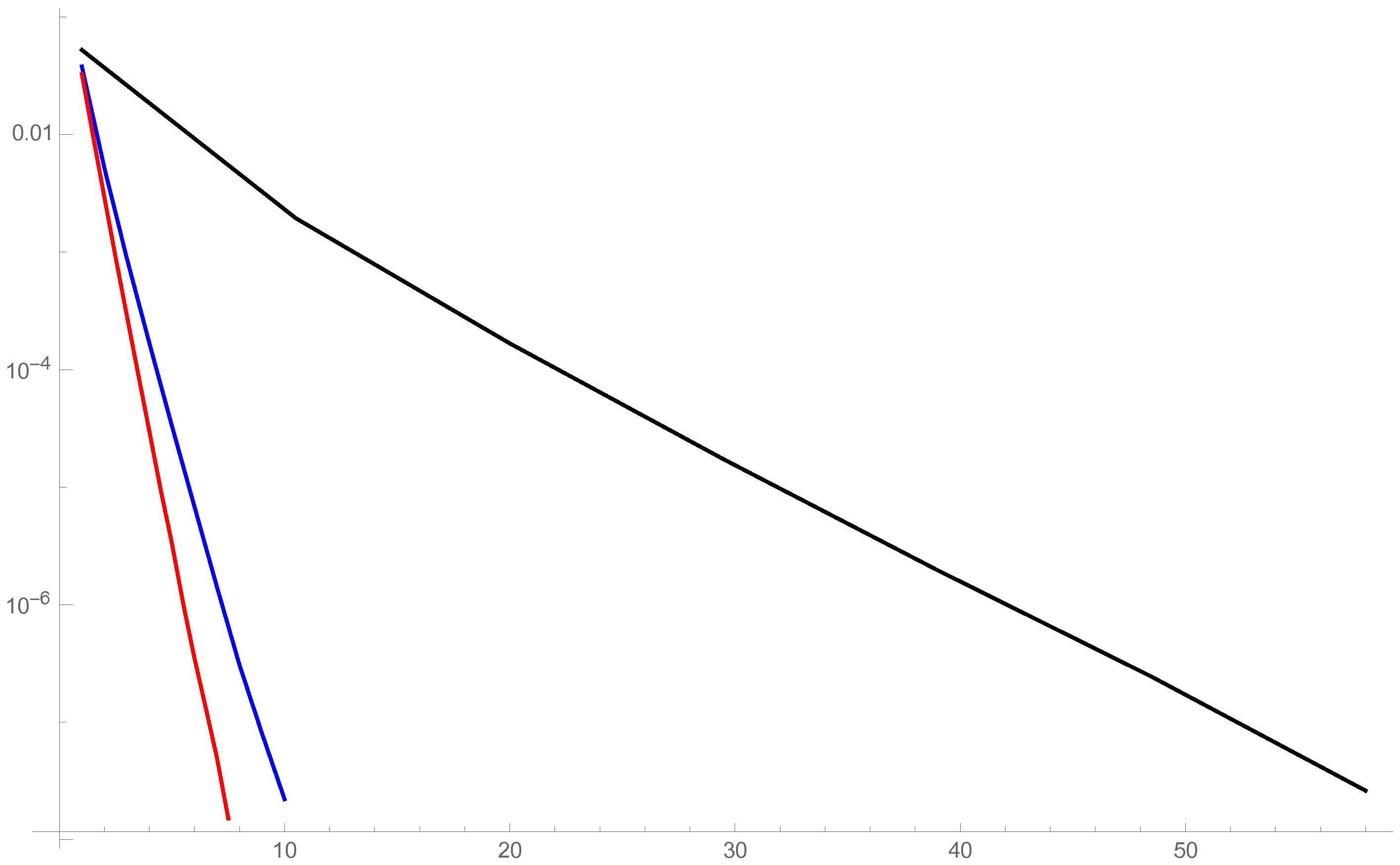
5. Illustration of the Results
5.1. Odd Case
5.2. Even Case
6. Conclusions
Author Contributions
Funding
Conflicts of Interest
References
- Fokas, A.S. A unified transform method for solving linear and certain nonlinear PDEs. Proc. R. Soc. Lond. A Math. Phys. Eng. Sci. 1997, 453, 1411–1443. [Google Scholar] [CrossRef]
- Fokas, A.S. On the integrability of linear and nonlinear partial differential equations. J. Math. Phys. 2000, 41, 4188–4237. [Google Scholar] [CrossRef]
- Fokas, A.S. A new transform method for evolution partial differential equations. IMA J. Appl. Math. 2002, 67, 559–590. [Google Scholar] [CrossRef]
- Biondini, G.; Wang, D. Initial-boundary-value problems for discrete linear evolution equations. IMA J. Appl. Math. 2010, 75, 968–997. [Google Scholar] [CrossRef]
- Deconinck, B.; Trogdon, T.; Vasan, V. The method of Fokas for solving linear partial differential equations. SIAM Rev. 2014, 56, 159–186. [Google Scholar] [CrossRef]
- Fokas, A.S. A Unified Approach to Boundary Value Problems; SIAM: Garden Grove, CA, USA, 2008. [Google Scholar]
- Pelloni, B. The spectral representation of two-point boundary-value problems for third-order linear evolution partial differential equations. Proc. R. Soc. Lond. A Math. Phys. Eng. Sci. 2005, 461, 2965–2984. [Google Scholar] [CrossRef]
- Pelloni, B.; Smith, D.A. Spectral theory of some non-selfadjoint linear differential operators. Proc. R. Soc. A Math. Phys. Eng. Sci. 2013, 469, 20130019. [Google Scholar] [CrossRef]
- Pelloni, B.; Smith, D.A. Evolution PDEs and augmented eigenfunctions. Half-line. J. Spectr. Theory 2016, 6, 185–213. [Google Scholar] [CrossRef] [Green Version]
- Smith, D.A. Well-posed two-point initial-boundary value problems with arbitrary boundary conditions. In Mathematical Proceedings of the Cambridge Philosophical Society; Cambridge University Press: Cambridge, UK, 2012; Volume 152, pp. 473–496. [Google Scholar]
- Fokas, A.S. Two-dimensional linear partial differential equations in a convex polygon. Proc. R. Soc. Lond. Ser. A Math. Phys. Eng. Sci. 2001, 457, 371–393. [Google Scholar] [CrossRef]
- Kalimeris, K. INITIAL and Boundary Value Problems in Two and Three Dimensions. Ph.D. Thesis, University of Cambridge, Cambridge, UK, 2010. [Google Scholar]
- Spence, E.A. Boundary Value Problems for Linear Elliptic PDEs. Ph.D. Thesis, University of Cambridge, Cambridge, UK, 2011. [Google Scholar]
- Batal, A.; Fokas, A.S.; Özsari, T. Uniform transform method for boundary value problems involving mixed derivatives. ar**s. J. Fluid Mech. 2012, 695, 288–309. [Google Scholar] [CrossRef]
- Fornberg, B.; Flyer, N. A numerical implementation of Fokas boundary integral approach: Laplace’s equation on a polygonal domain. Proc. R. Soc. A Math. Phys. Eng. Sci. 2011, 467, 2983–3003. [Google Scholar] [CrossRef] [Green Version]
- Grylonakis, E.N.G.; Filelis-Papadopoulos, C.K.; Gravvanis, G.A. A class of unified transform techniques for solving linear elliptic PDEs in convex polygons. Appl. Numer. Math. 2018, 129, 159–180. [Google Scholar] [CrossRef]
- Hashemzadeh, P.; Fokas, A.S.; Smitheman, S.A. A numerical technique for linear elliptic partial differential equations in polygonal domains. Proc. Math. Phys. Eng. Sci. 2015, 471, 20140747. [Google Scholar] [CrossRef]
- Trogdon, T.; Biondini, G. Evolution partial differential equations with discontinuous data. Q. Appl. Math. 2019, 77, 689–726. [Google Scholar] [CrossRef]
- Lamé, G. Mémoire sur la propagation de la chaleur dans les polyèdres, et principalement dans le prisme triangulaire régulier. J. I’Ecole Poly Tech. 1833, 22, 194–251. [Google Scholar]
- Fokas, A.S.; Kalimeris, K. Eigenvalues for the Laplace operator in the interior of an equilateral triangle. Comput. Methods Funct. Theory 2014, 14, 1–33. [Google Scholar] [CrossRef]
- Pinsky, M.A. The eigenvalues of an equilateral triangle. SIAM J. Math. Anal. 1980, 11, 819–827. [Google Scholar] [CrossRef]
- Pinsky, M.A. Completeness of the eigenfunctions of the equilateral triangle. SIAM J. Math. Anal. 1985, 16, 848–851. [Google Scholar] [CrossRef]
- Práger, M. Eigenvalues and eigenfunctions of the Laplace operator on an equilateral triangle. Appl. Math. 1998, 43, 311–320. [Google Scholar] [CrossRef] [Green Version]
- Terras, R.; Swanson, R. Image methods for constructing Green’s functions and eigenfunctions for domains with plane boundaries. J. Math. Phys. 1980, 21, 2140–2153. [Google Scholar] [CrossRef]
- McCartin, B.J. Eigenstructure of the equilateral triangle, Part I: The Dirichlet problem. Siam Rev. 2003, 45, 267–287. [Google Scholar] [CrossRef]
- McCartin, B.J. Eigenstructure of the equilateral triangle, Part II: The Neumann problem. Math. Probl. Eng. 2002, 8. [Google Scholar] [CrossRef]
- McCartin, B.J. Laplacian Eigenstructure of the Equilateral Triangle; Hikari Limited: Rousse, Bulgaria, 2011. [Google Scholar]


© 2020 by the authors. Licensee MDPI, Basel, Switzerland. This article is an open access article distributed under the terms and conditions of the Creative Commons Attribution (CC BY) license (http://creativecommons.org/licenses/by/4.0/).
Share and Cite
Kalimeris, K.; Fokas, A.S. The Modified Helmholtz Equation on a Regular Hexagon—The Symmetric Dirichlet Problem. Axioms 2020, 9, 89. https://doi.org/10.3390/axioms9030089
Kalimeris K, Fokas AS. The Modified Helmholtz Equation on a Regular Hexagon—The Symmetric Dirichlet Problem. Axioms. 2020; 9(3):89. https://doi.org/10.3390/axioms9030089
Chicago/Turabian StyleKalimeris, Konstantinos, and Athanassios S. Fokas. 2020. "The Modified Helmholtz Equation on a Regular Hexagon—The Symmetric Dirichlet Problem" Axioms 9, no. 3: 89. https://doi.org/10.3390/axioms9030089