1. Introduction and Background
Alzheimer’s disease (AD) is a neurological disease that slowly destroys brain cells, resulting in reduced memory, cognitive abilities, and daily function. It is a complicated illness that progresses gradually. This leads to brain cell death, which gradually impairs an individual’s capacity to complete tasks and causes loss of memory and thought [
1]. Dementia is the result of the disease’s effects on cognitive function. One example of a neurodegenerative illness that not only affects localized grey matter but also results in improper integration across different sections of the brain is Alzheimer’s disease [
2].
Presently, around 90 million individuals are affected by AD, and projections indicate that by 2050, the number of AD patients will be increased to 300 million [
3]. Alzheimer’s disease develops in three stages, beginning with showing some symptoms of memory impairment, called mild cognitive impairment (MCI). As it progresses to each subsequent stage, the disease becomes more severe, and patients experience difficulty performing everyday tasks. Studies [
4,
5,
6,
7] have conducted research to determine which particular parts of the brain are impacted by AD. The study [
8] conducted research on AD to explore those aspects of AD which are not covered by the previous literature. As a result, the goal of their groundbreaking research is to examine the afflicted brain areas at each stage of AD. They also classify AD patients into three groups based on their MCI status: mild, moderate, and severe.
The study [
8] conducted research on AD to explore those aspects of AD which are not covered by the previous literature. Therefore, the objective of the research, which is novel, is to analyze the affected brain regions during each stage of AD. The authors also perform binary classification between MCI and mild, MCI and moderate, and MCI and severe stage of AD patients. Similarly, ref. [
9] used a support vector machine (SVM) learning algorithm to distinguish AD from healthy control (HC) and MCI from HC by considering data from 52 HCs patients, 99 MCI patients, and 51 AD patients. Alzheimer’s disease was classified with 93.2 percent accuracy in healthy controls, while mild cognitive impairment was classified with 76.4 percent accuracy in healthy controls.
The authors used classical classification methods SVM, K-near neighbor (KNN), and Naive Bayes (NB) to classify healthy and AD patients in [
10]. The data include brain scans from 416 people aged between 18 and 96 years. The analysis showed that the SVM could classify normal brains from Alzheimer’s brains with 95 percent accuracy. NB and KNN, on the other hand, delivered 90 percent accuracy for the data used for experiments.
The authors in [
11] observed during their research that Alzheimer’s disease affects the entire brain and that the regions with the most significant differences are the posterior cingulate cortex (PCC), middle temporal gyrus (MTG), entorhinal cortex, and hippocampus. The author employed machine learning methods SVM, linear discriminant analysis (LDA), artificial neural network (ANN), and logistic regression (LR) to classify AD stages using resting-state fMRI data. The authors considered three stages of AD, including mild, moderate, and severe, and used machine learning algorithms to identify different stages of AD.
The study [
12] examines various machine learning architectures to distinguish AD from mild cognitive impairment (MCI). DenseNet-169 emerges as the top performer, achieving an impressive 82.2% accuracy in AD classification from MCI. Similarly, the authors explore health records using manifold learning techniques to differentiate early-stage AD groups [
13]. Various methods, such as spectral embedding and autoencoder-based manifolds, are applied to the ADNI dataset for insightful analysis.
In [
14], a pioneering deep learning model known as FDN-ADNet is introduced. The model aims to enhance early AD diagnosis by extracting features across hierarchical levels. It employs a Fuzzy Hyperplane-based least square twin support vector machine (FLS-TWSVM) classification technique and uses sagittal plane slices from 3D MRI images to train the FDN-ADNet model. With impressive classification accuracy rates of 97.15% for CN vs. AD, 97.29% for CN vs. MCI, and 95% for AD vs. MCI, the model excels in distinguishing cognitive states. This approach shows potential as a robust tool for early AD diagnosis.
Sadiq et al. [
15] introduced an automated framework that addresses existing limitations through a comprehensive exploration of signal decomposition, feature selection, and neural network methods. By achieving substantial enhancements of up to 26.1% and 26.4% compared to current state-of-the-art approaches, this framework holds potential for both subject-dependent and independent brain–computer interface (BCI) systems. It offers a pathway for the creation of adaptable BCI devices, catering to motor-disabled users’ interaction needs. Similarly, ref. [
16] introduces an innovative automated computerized framework to effectively detect motor and mental imagery (MeI) EEG tasks. The approach leverages empirical Fourier decomposition (EFD) and improved EFD (IEFD) techniques. The EEG data are initially denoised using multiscale principal component analysis (MSPCA), followed by EFD to decompose nonstationary EEG into modes. The IEFD criterion facilitates the selection of a distinct mode. Time- and frequency-domain features are then extracted and classified using a feedforward neural network (FFNN) classifier.
The study [
17] utilizes the multivariate variational mode decomposition (MVMD) on 18-channel EEG data from the motor cortex, along with the Relief-F feature selection technique, yielding remarkable results. In subject-dependent experiments, the approach achieved an average classification accuracy of 99.8%. For subject-independent experiments, the accuracy reached 98.3%. Moreover, this combination consistently delivered accuracy exceeding 99% for subjects with either ample or limited training samples, across both subject-dependent and independent scenarios. These impressive outcomes underscore the framework’s adaptability for subject-specific and subject-independent BCI systems.
The authors proposed a framework in [
18] which consists of three main phases: firstly, investigating the chaotic nature of EEG signals through phase space dynamics visualization; secondly, extracting thirty-four graphical features to decode chaotic patterns in normal and alcoholic EEG signals; thirdly, selecting optimal features using various techniques combined with machine learning and neural network classifiers. Results show that the method achieves remarkable classification performance, with 99.16% accuracy, 100% sensitivity, and 98.36% specificity. The combination of Henry gas solubility optimization and feedforward neural network stands out as the most effective approach.
The study [
19] employs multiscale principal component analysis for robust noise reduction in the preprocessing phase. A novel automated strategy for channel selection is introduced and validated through comprehensive comparisons of decoding methods. The study pioneers the use of MEWT to capture joint amplitude and frequency components, enhancing Motor Imagery applications. The study applies a robust correlation-based feature selection technique to reduce system complexity and computational demands.
Akbari et al. [
20] introduces a novel strategy to diagnose depression using geometric features extracted from EEG signal shapes via second-order differential plots (SODPs). Various geometric characteristics are derived from the SODPs of normal and depressed EEG signals. Binary particle swarm optimization selects relevant features, which are then used with SVM and k-nearest neighbor classifiers to identify depression accurately. This approach capitalizes on the distinctive geometric properties of EEG signals to improve depression diagnosis. Similarly, ref. [
21] proposes novel geometric features for distinguishing between seizure (S) and seizure-free (SF) EEG signals. The features are derived from the Poincaré pattern of discrete wavelet transform coefficients, utilizing distinct plot patterns. These features, including 2D projection descriptors (STD), triangle area summation (STA), the shortest distance from the 45-degree line (SSHD), and the distance from the coordinate center (SDTC), aid in classifying EEG signals accurately.
The study [
22] used a Gaussian process (GP) machine learning algorithm to classify MCI and AD. The authors applied the GP model to 77 subjects, 50 MKI and 27 AD. All subjects had resting-state fMRI data. Experimental results demonstrate a 97 percent accuracy for GP and observed that GP performs effectively in MCI and AD classification. Ref. [
23] used SVM, LDA, and logistic regression (LR) to classify susceptible brain regions associated with Alzheimer’s disease. They used predefined regions of the AD hippocampus, MTG, PCC, and entorhinal cortex. They did not define regions with independent component analysis (ICA). The study’s goal was to identify brain areas implicated in various phases of Alzheimer’s disease. Independent component analysis (ICA) was used to extract information from mixed data from fMRI data in order to localize specific brain areas affected by distinct stages of AD. The author used SPM12 to extract voxel data for the associated brain areas at each stage when applying ICA to specify brain regions. SPM12 implements a generalized linear model (GLM) applied to each voxel of a functional image. The voxel data extracted in the previous step were further used for multi-class classification of the stages using machine learning algorithms.
In contrast to earlier studies, the goal of this study is to investigate the regions of the brain that are impaired at each stage of the formation of AD. Six affected brain regions with moderate cognitive impairment were examined, four in the preliminary stages of AD and six each in the subsequent stages. The precuneus, cuneus, middle frontal gyri, calcarine cortex, superior medial frontal gyri, and superior frontal gyri were common brain areas affected by all these stages. The brain activations vary among all these stages. Brain activation reduces as the stages progress.
Functional change in one patient varies from one stage to the other. If the patient data have changed in each stage, then it is not possible to observe the functional changes in all four stages. To observe the functional changes in all four stages, the data include brain scans from the same 18 individuals for all four stages. The voxels have been extracted from the six affected brain regions. These regions were defined by the regional changes during all four stages. Data from the same patients for all four stages are not available.
This study used four stages by including healthy diseases of the same patients for multi-class classification. To the best of our knowledge, we are the first to classify our dataset into multiple stages with the selected specific regions using machine learning models. The healthy stage, the early stage, and the end stage of AD were the main classification pillars. For the multi-class classification, we selected the same patients in the four phases of AD.
Despite the contribution of the above-discussed studies, this study still lacks high-accuracy models. Machine learning models are not very well investigated for Alzheimer’s disease regarding their use at different levels of AD and the influence of AD on different regions of the brain. In this regard, this study applies eight machine learning models, both linear and nonlinear, which include neural networks, linear SVM, polynomial SVM, nearest neighbors, decision trees (DT), random forests (RF), AdaBoost, and NB. The primary objective is to find specific brain regions affected at any stage of AD based on fMRI data. To extract brain morphological patterns, all machine learning algorithms successfully classified AD patients using data from selected regions with a satisfactory classification accuracy of more than 90%. Experimental results show that AdaBoost and KNN techniques achieve high classification accuracy (98%) and perform well on this particular dataset.
This study is further divided into three sections.
Section 2 presents the proposed methodology and explains different phases of the approach adopted for experiments. Results and analysis are presented in
Section 3, while
Section 4 provides discussions. In the end,
Section 5 concludes this study.
3. Results and Analysis
After data preprocessing, we looked at the brain regions in MCI, including mild, moderate, and severe AD stages that were active at rest. Using the Group ICA Toolbox, these regions were retrieved using independent component analysis. Experiments are performed using an 80-20 split, where 80% of the data are used for model training and 20% are used for testing the models. A 10-fold cross-validation is used in this study.
3.1. Affected Brain Region Identification
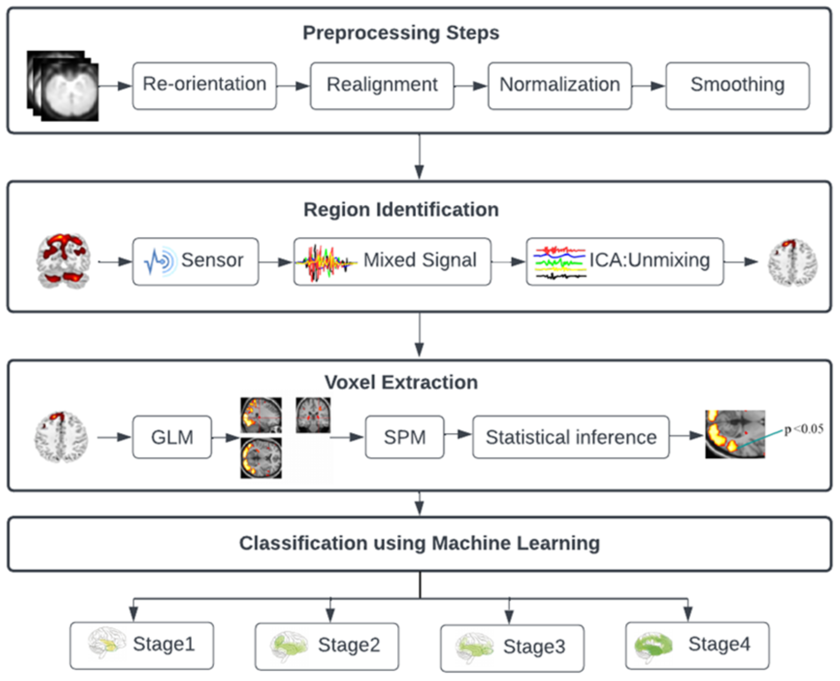
In the initial phase of data analysis, the application of group-independent component analysis (ICA) is employed on fMRI data to extract insights from mixed data. The objective is to precisely identify the distinct brain regions impacted at various stages of AD. ICA, also referred to as the blind source separation (BSS) method, serves as a powerful tool for revealing hidden sources or factors that contribute to data, including those in fMRI. This technique has found extensive use in uncovering independent sources underlying complex information. In this study, by utilizing the ICA approach, a total of 20 brain regions are discerned across the four AD stages, each of which is associated with the disease progression within the dataset of 18 subjects.
Following data preprocessing, we used the Group Independent Component Analysis Toolbox (GIFT) to pinpoint the areas of the brain in people with MCI, including mild, moderate, and severe AD, that were active when they were at rest. These regions were recovered using independent component analysis (ICA), and GIFT provided peak coordinates for each component. Only the active brain areas are identified by GIFT; the precise name of each given region is not provided. Only the peak MNI coordinate of that specific location is provided. The GIFT toolbox’s MNI coordinates and anatomical automated labeling (aal. nii) were utilized to determine the name of a specific region. We identify the particular region by using MRIcron and peak coordinates in the MNI field.
MCI affected brain areas including the cuneus, precuneus, parahippocampal, frontal middle gyrus, putamen, and frontal superior gyrus. The calcarine cortex, frontal superior medial gyrus, frontal middle gyrus, and cuneus are the brain areas that are moderately affected. The calcarine cortex, precuneus, parahippocampal, frontal superior medial, frontal superior, and middle temporal gyri are affected brain areas in the severe stage of AD.
Affected brain regions in MCI include the cuneus, precuneus, parahippocampal, frontal middle gyrus, putamen, and frontal superior gyrus. Affected brain regions at the moderate stage are the calcarine cortex, frontal superior medial gyrus, frontal middle gyrus, and cuneus. Affected brain regions at the severe AD stage are the calcarine cortex, precuneus, parahippocampal, frontal superior medial gyrus, frontal superior gyrus, and middle temporal gyrus.
Figure 2 shows the brain regions that are active at rest in the early stages of MCI, including mild, moderate, and severe stages of AD, shown from an orthogonal perspective. Each region is assigned a different color, and the legends located at the bottom right of the image indicate the corresponding names of the brain regions. This orthogonal view is manually generated using features of MRICron.
3.2. Voxel Data Extraction
The voxel data for the appropriate brain areas were extracted at each stage using SPM12 when the brain regions were identified using ICA. Subsequently, the data analysis phase entailed the implementation of the general linear method (GLM). This technique enabled the extraction of voxels from the previously identified brain regions. Voxels, indicative of volume measurements within imaged structures, were used to pinpoint specific areas of interest. The activations within these identified brain regions displayed unique patterns across each AD stage. The corresponding numerical values representing these activations were meticulously recorded and are provided in tabular format within the paper.
First, we computed the mean image to aggregate the data from each subject. In other words, the 105 photos of each patient were added together. Then, using the labels provided in SPM12, the first level analysis was carried out and voxel data of specific regions were collected. The following specifications must first be given in order to extract data.
3.2.1. Model Specification
Before further analyzing fMRI data, the design matrix must be specified first. Several choices can be made depending on the conditions in the experiment. In the model specification, we need to set the output directory, data to be analyzed, inter-scan interval, scans per session, number of conditions, and the onset value. These values require a fixed model to run. The model specification will generate a file with the name spm.mat in the specified directory that will be used for further analysis.
Figure 3 below shows the design matrix of a single AD patient at stage 1. Since the data were in a resting state, only one condition was set. The grey represents when the condition was on, and the white represents when the condition was set off. Similar design matrices were constructed at the second, third, and fourth stages for voxel data extraction.
3.2.2. Model Estimation
The next step is to perform model estimation when the model is specified for the analysis. This is accomplished by selecting the spm.mat file from the directory. After execution, it will display a summary of the design matrix and parameters.
3.2.3. Displaying Results
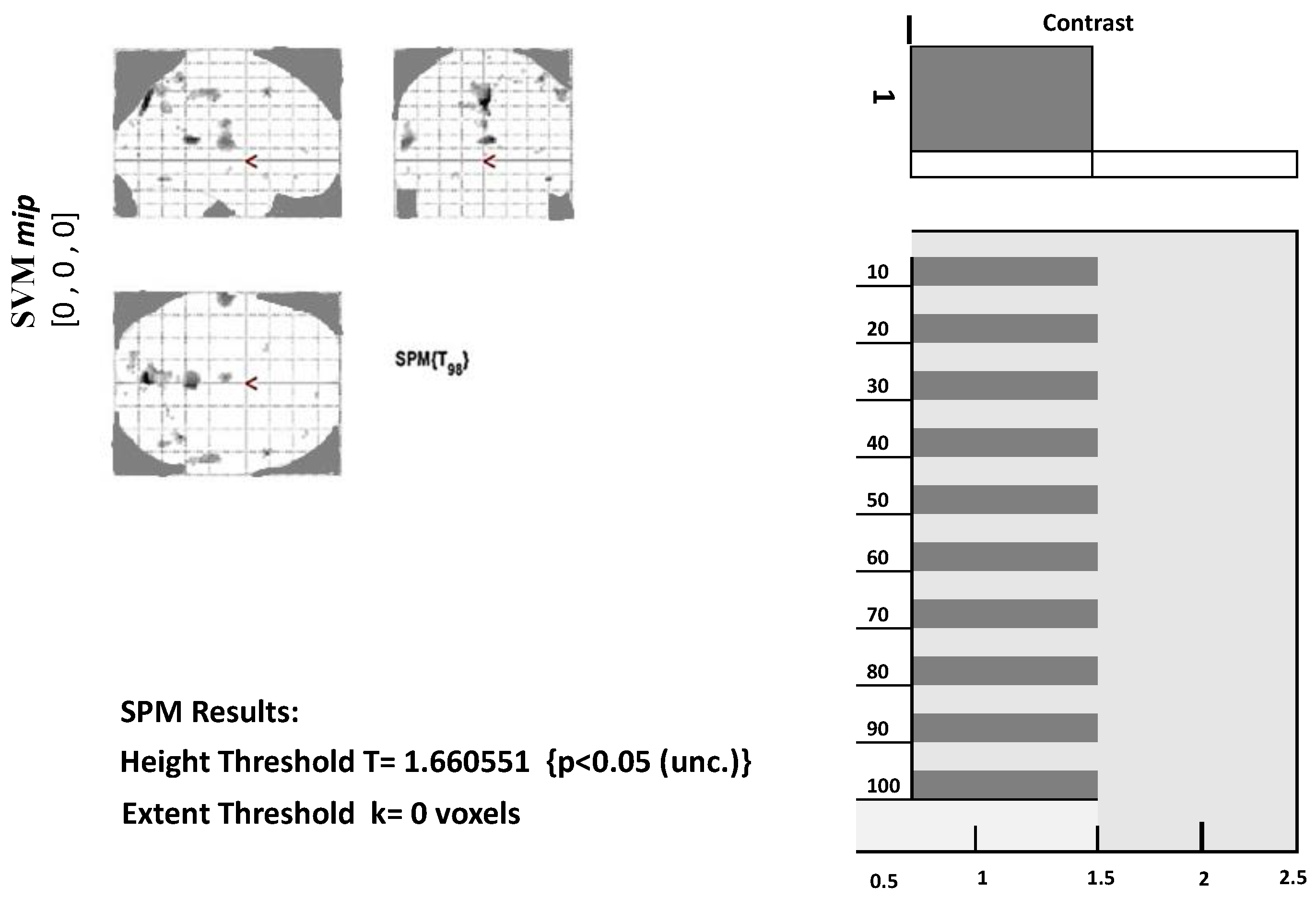
We first need to define a contrast to view the results from model estimation. Contrast may be set according to conditions involved in the experiment. In determining contrast, use 1 for the most active condition, a negative number for the less active condition, and 0 for the condition to be ignored. Next, we need to set a threshold for the set mask. The smaller the threshold value, the more significant the voxel will appear. We also need to place an extended threshold value, which means the minimum number of voxels in each cluster.
Figure 3 below displays a glass brain view in which activated clusters/brain regions are marked with grey and black dots.
Along with the glass brain view, the
p-value for the highly significant voxels of each cluster can also be obtained. Also, for each voxel, we can extract its values, as given in
Table 3.
Table 3 shows the number of voxels of 22 brain regions. The first level analysis was carried out, and voxel data for the targeted regions were extracted using the labels from SPM12.
The process of choosing particular brain regions or voxels of interest in neuroimaging studies is driven by a combination of scientific rationale and practical considerations. Researchers make these selections based on the specific hypotheses they aim to test, the existing body of knowledge in the field, and the underlying neurobiology of the condition under investigation. This process is integral to the study’s success, influencing the clarity of results and the ability to draw meaningful conclusions.
Table 4 presents the results attained by machine learning algorithms that were considered for classification. Considering the presented results, the overall performance of AdaBoost is better than all other models, with an average accuracy of 96.36% and precision, recall, and F1 scores of 96.50%, 95.50%, and 96.5%, respectively, followed closely by RF, with accuracy, precision, recall, and F1 scores of 93.27%, 95%, 93.5%, and 94%, respectively.
Figure 4 given above presents the comparative accuracy values. From the presented results, it can be seen that Adaboost and RF dominate other implemented machine learning algorithms. Therefore, the AdaBoost method is superior to the implemented machine learning algorithms.
3.3. Performance Comparison with Existing Studies
A performance analysis is also carried out to compare the performance of this study’s results with existing studies. For this purpose, [
23,
32,
33,
34,
35] are selected because these studies also perform Alzheimer’s disease detection using the same dataset. These studies employed various machine learning models like SVM, AdaBoost, KNN, RF, etc.
Table 5 shows the comparison of the results regarding reported accuracy. It can be observed that the results obtained in the current study are superior to those in the existing studies.
3.4. Relevance to Research Objectives
The brain regions or voxels chosen for analysis are often directly related to the research objectives. Researchers target areas known to be functionally or structurally linked to the cognitive processes or behaviors they intend to explore. For example, in studies of mood disorders, the amygdala and prefrontal cortex might be of particular interest due to their roles in emotional regulation.
3.4.1. Prior Research
Existing literature plays a vital role in guiding the selection of brain regions. This study is built on previous studies that have identified specific regions as crucial for certain functions or implicated in the disorder being studied. This iterative process helps to advance knowledge and build a cohesive understanding of the brain’s complexities.
3.4.2. Neurobiological Significance
Selections are often grounded in the known neurobiological relevance of specific regions. If a study pertains to sensory processing, brain areas associated with sensory modalities are natural choices. This ensures that the analysis aligns with the underlying neural processes.
3.5. Practical Considerations
Statistical Considerations: Focusing on specific regions mitigates the multiple comparisons problem, reducing the risk of false positives. By narrowing the scope of analysis, researchers enhance the statistical power of their findings.
Data Availability: Practical constraints, such as the scope of available imaging data or the research question’s focus, might dictate which regions are feasible to analyze.
Analysis Complexity: Targeting specific regions simplifies the analysis process and aids in result interpretation. Analyzing a vast number of regions can lead to overfitting and complicate the interpretation of findings.
Interpretation Clarity: Concentrating on selected brain regions enhances the interpretability of results. Researchers can provide more precise explanations and insights, facilitating a deeper understanding of the study’s implications.
3.6. Impact on Results
The decision to narrow the focus to specific brain regions has substantial ramifications for the study’s outcomes:
Localization Precision: By concentrating on certain regions, researchers achieve higher spatial resolution, enabling a more accurate understanding of the neural underpinnings of behavior or cognitive functions.
Sensitivity and Specificity: Focusing on particular regions can heighten the sensitivity to detect subtle effects within those areas. However, this specificity might reduce the model’s ability to detect effects in other regions.
Generalizability: While the selected regions provide detailed insights, the findings might not be universally applicable to the entire brain or broader neural networks.
Potential Insights Missed: Overly specific region selection could overlook relevant interactions or compensatory mechanisms occurring in other brain areas.
Interpretational Bias: The choice of regions could introduce bias, influencing the interpretation and presentation of results.
In summary, the process of selecting specific brain regions or voxels of interest is a carefully considered decision that balances scientific intent, statistical power, and practical feasibility. These selections play a pivotal role in determining the study’s outcomes, influencing the accuracy of localization, sensitivity to effects, generalizability, and potential insights gleaned from the analysis.
3.7. Limitations and Future Work
While leveraging identified brain regions and their classification for AD, diagnosis, and prognosis offers promising avenues, there exist important limitations that call for consideration. The translation of intricate neuroimaging data into meaningful clinical insights remains a challenge, necessitating robust interdisciplinary cooperation among clinicians, data scientists, and neuroscientists. Moreover, the variability intrinsic to brain anatomy and imaging techniques introduces potential disparities that can impact the reliability of findings across studies.
In the pursuit of clinical applicability, bridging the gap between research discoveries and practical healthcare implementation becomes paramount. Develo** user-friendly tools and decision support systems that harness brain region classification could empower clinicians with actionable insights for patient care. Additionally, the potential emergence of interventions targeting specific brain regions could redefine treatment strategies, potentially revolutionizing patient outcomes.
In essence, while the integration of brain region identification and classification holds immense potential, addressing challenges surrounding data interpretation, variability, and ethical considerations remains crucial. The trajectory of AD research will likely entail embracing advanced methodologies, adopting personalized approaches, and fostering seamless interdisciplinary collaboration to steer the field toward enhanced diagnosis, prognosis, and transformative treatment interventions within clinical settings.
4. Discussion
A neurological encephalopathy that is progressive and incurable is AD. The brain’s regional grey matter as well as areas especially linked to memory and cognitive behavior are damaged by AD. The veracity of these areas has been investigated and confirmed by numerous surveys. The hippocampus is the area of the brain that is affected by AD, according to [
36]. The temporal lobe, insula, and posterior cingulate/precuneus are a few of the brain regions that show deterioration in grey and white matter in those migrating from MCI to AD [
5]. Similar findings are made by [
6], who discovered that neurodegeneration begins in the entorhinal cortex and hippocampus before spreading to other frontal, temporal, and parietal regions that are damaged by AD. The study in [
7] reported decreased functional connectivity between the hippocampus and a number of brain regions, including the middle temporal gyrus, precuneus, inferior temporal cortex, medial frontal cortex, superior temporal cortex, and posterior cingulate gyrus. Additionally, they saw an improvement in the functional connection between the left hippocampus and the lateral prefrontal cortex.
By identifying the exact brain regions impacted at each stage of AD, the current study fills a gap in the body of prior literature. The GIFT Toolbox v4.0 of MATLAB was used to implement ICA. In order to determine whether brain regions related to working memory are impacted, Chatterjee et al. [
26] employed GIFT to run ICA on fMRI data in cases of schizophrenia. Each subject’s 13 ICs were taken into account. After ICs were identified, the associated brain region was marked using the automated anatomical labeling (AAL) atlas. The most frequent ICs were identified as the brain regions that experience schizophrenia issues in their conclusion. Similar directions are taken by this present study, which involved four stages, looking at fMRI data from each patient at MCI, stage 1, stage 2, and stage 3 of AD. Each patient’s fifteen (15) ICs were examined, and those without a recognizable pattern were eliminated. The AAL atlas in the mricron32 program was used to identify the matching brain regions for the remaining ICs, and the generated ICs were validated using related techniques.
Most studies are conducted on MRI data which are structural data. Deep learning algorithms are highly recommended to analyze structural data because they compute structural changes in brain structure more efficiently than machine learning algorithms. We used fMRI data for our research, which are functional data. Localizing disease is a complicated task in fMRI data. Utilizing cutting-edge neuroimaging modalities such as fMRI, researchers can meticulously examine the intricate structural and functional changes unfolding within the brain. This scrutiny unveils subtle alterations that might precede noticeable symptoms of AD. Focused analysis of specific brain regions, notably the hippocampus, and select cortical areas typically vulnerable to the disease, can unveil incipient atrophy and functional anomalies, thereby facilitating early detection.
A statistical algorithm such as ICA makes it easy to identify the location of each component/brain region, and the brain region name is then identified using the MRICron tool. After identifying regions, we use GLM to extract the voxel means, a numeric value of activation of brain regions at each stage of AD. Brain region activation detail is in numeric form and the detail of activation is not too large. For smaller amounts of data and for precise computation, machine learning algorithms are better than deep learning algorithms. For this reason, this study employed machine learning algorithms. We intend to apply ensemble models and other advanced variants of machine learning models in future work.
Data leakage is an important concern for studies focusing on Alzheimer’s disease and several causes can lead to data leakage, as pointed out by [
37]. For example, not splitting the dataset at the subject level may lead to data leakage. Samples from the same subject may appear in training, testing, and validation sets. Similarly, data augmentation before train–test splits may lead to similar data appearing in different sets. Biased transfer learning and lack of an independent test set are also attributed to data leakage. This study considered the data from the same subject for different stages of Alzheimer’s, which poses a risk of data leakage. However, the data from subjects are split for each stage separately, which removes the risk of data leakage at the subject level. A train–test split is used to make an independent test set comprising 20% of the data to avoid data leakage at this stage. No use of transfer learning and data augmentation also reduces the risk of data leakage in this study. K-fold cross-validation further corroborates the validity of the results.

 ,
, 


