
Multi-UAV Optimal Mission Assignment and Path Planning for Disaster Rescue Using Adaptive Genetic Algorithm and Improved Artificial Bee Colony Method

 ,
,
Abstract
:1. Introduction
2. Problem Formulation
3. Optimization Modelling and Its Solution
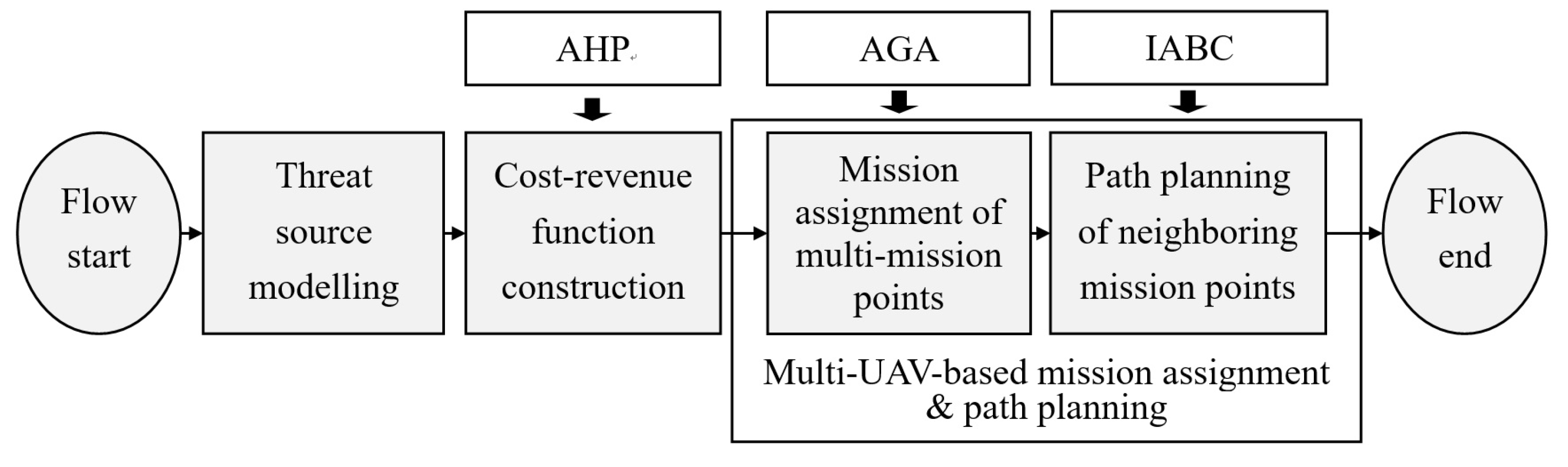
3.1. The Proposed Computational Flow Chart
3.2. The Threat Source Modelling Methods
- (1)
- The severe weather threat source
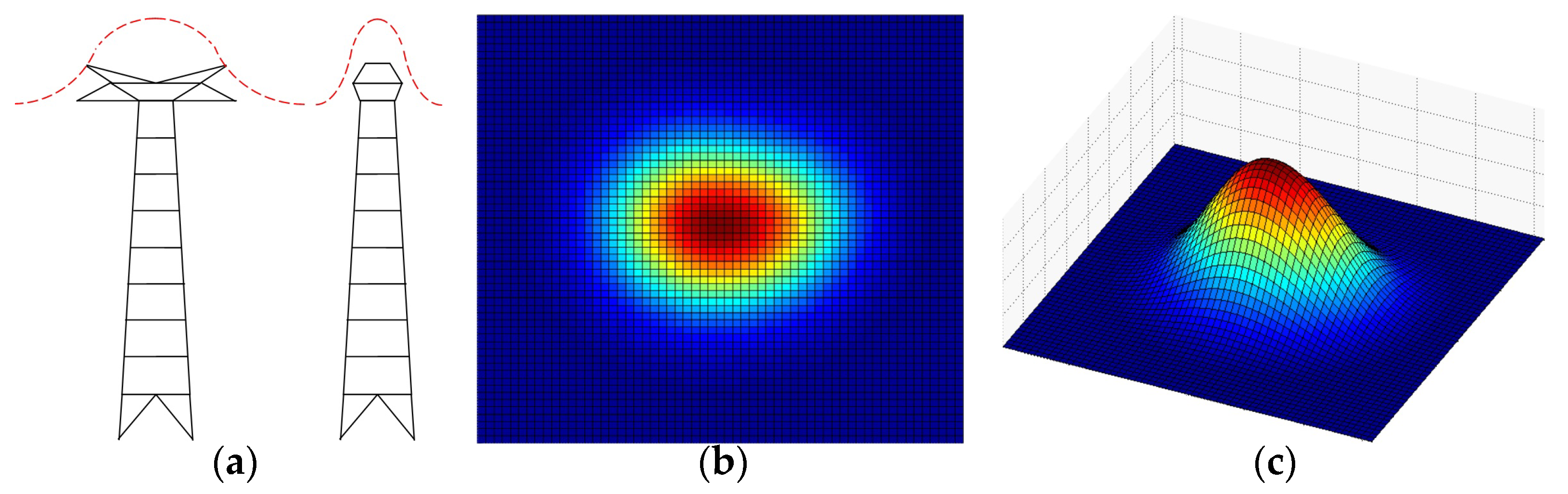
- (2)
- The transmission tower threat source
- (3)
- The upland threat source
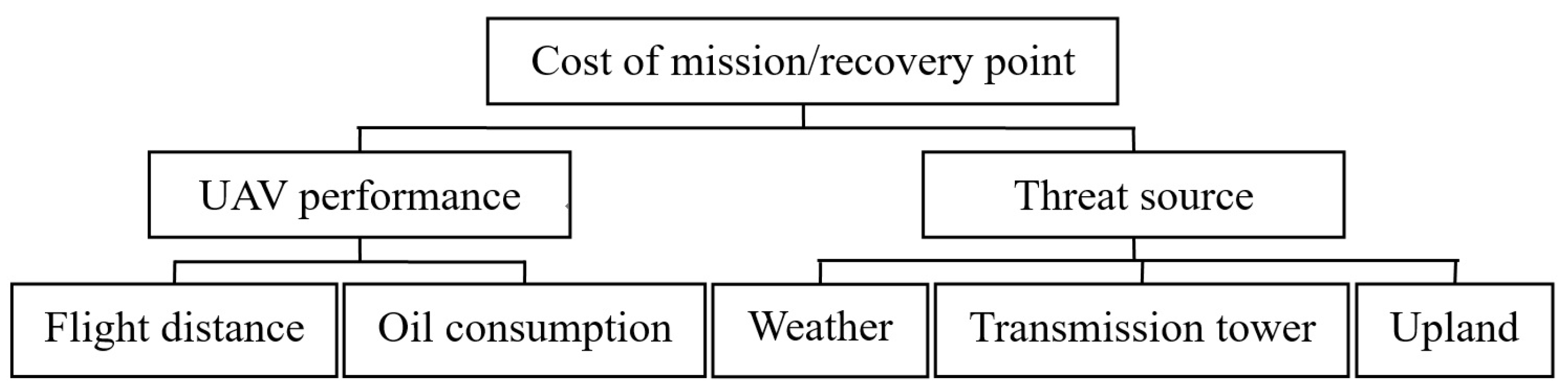
3.3. The Cost-Revenue Function
3.4. The Optimal Computational Methods: AGA and IABC
- (1)
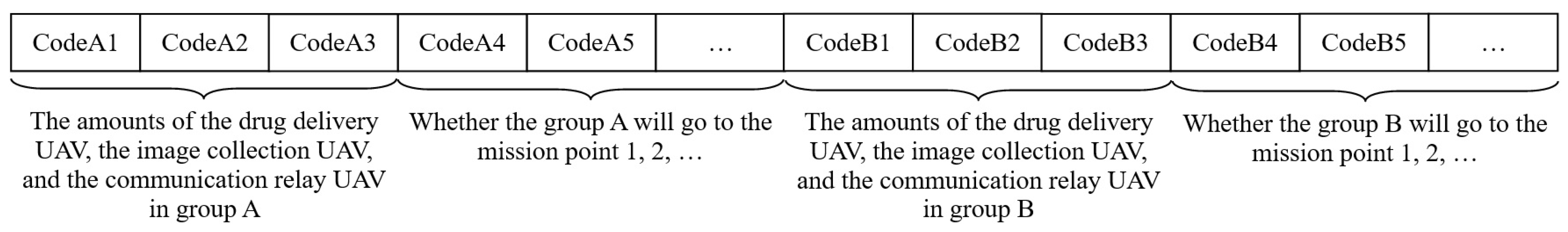
- The optimal mission assignment of multiple mission points using AGAThe multi-UAV can be allocated into different UAV groups by AGA to accomplish the rescue task. The computational steps of AGA are listed below.
- (a)
- The population initialization. The initial population is generated, i.e., a series of initial solutions of mission assignment are created by the random number. The population size N_AGA, the current iteration number p_AGA, the maximum iteration number p_AGAmax, the crossing probability Pp_AGA,C, and the mutation probability Pp_AGA,M etc., are set.
- (b)
- The fitness function calculation [44]. The calculation method of the fitness function is shown by Equation (16).where fp_AGA is the fitness function in the p_AGAth iteration; T2p_AGA is defined in (15).
- (c)
- The iterative computation of AGA. Three kinds of computations are implemented [45]: the selection operation, crossover operation, and mutation operation. First, the selection operation considers the estimation result of fitness function, and its probability is defined in Equation (17). The roulette wheel selection method is utilized in this study. Second, the crossover processing is carried out by exchanging several gene fragments at the positions of two randomly selected individuals. Third, the mutation step is achieved by switching two genes of one randomly selected individual. The probabilities of crossover and mutation operations are defined in (18) and (19).where Pp_AGA,S is the selection probability; fp_AGA is the fitness function in the p_AGAth iteration; N_AGA is the maximum population number; Pp_AGA,C is the cross probability; ap_AGA, bp_AGA, cp_AGA, and dp_AGA are the control parameters in the p_AGAth iteration, ap_AGA = 1.0, bp_AGA = 1.2, cp_AGA = 1.0, and dp_AGA = 1.35 in this study; Pp_AGA,C_max is the maximum of cross probability; fp_AGA,max is the maximum of fitness function; fp_AGA,mean is the mean of fitness function; Pp_AGA,M is the mutation probability; Pp_AGA,M_max is the maximum of mutation probability.
- (2)
- The optimal path planning between neighboring mission points using IABCAn IABC algorithm is used to find the optimal path between neighboring mission points. The basic computational steps of artificial bee colony (ABC) algorithm are presented below.
- (a)
- The population initialization. The random solutions of ABC algorithm are created. The corresponding computation method [47] can be written by (23). The maximum iteration is also set, and the initial iteration number is 0.where xij is the coordinate of flight path; xjmin and xjmax are the minimum and maximum values of xij; i = 1, 2, …, NP, and NP is the total number of bees; j = 1, 2, …, D. Here D is the dimension of estimated parameter, D = 2 in this study.
- (b)
- The path updating of employed foragers. First, the solutions vij of employed foragers can be computed by (24), and then the fitness function will be estimated. Here, the fitness function uses the cost-revenue function in Equation (14) to estimate its fitness degree by Equation (25). The classical greedy algorithm [48] is used to select the proper solution. Second, the probability Pp_IABC is calculated by (26) and the corresponding scouter can be selected properly. Third, the solution vij of the onlooker from the solutions xij selected depending on Pp_IABC will also be computed by (24); and the greedy algorithm will be used again to select the proper solution. Fourth, the abandoned solution of scouter will be determined, and a new randomly solution will be considered for them. Fifth, the best solution will be recorded in this round and the iteration counter will be added by 1.where i = 1, 2, …, NP; j = 1, 2, …, D, and k = 1, 2, …, NP; k and j are the randomly chosen indexes, and k ≠ i; fp_IABC is the fitness function of solution which is proportional to the nectar amount; T1p_IABC is the cost-revenue function of the p_IABCth iteration.
- (c)
- The iteration computation will be terminated if the iteration counter reach its upper limitation.
4. Results and Discussions
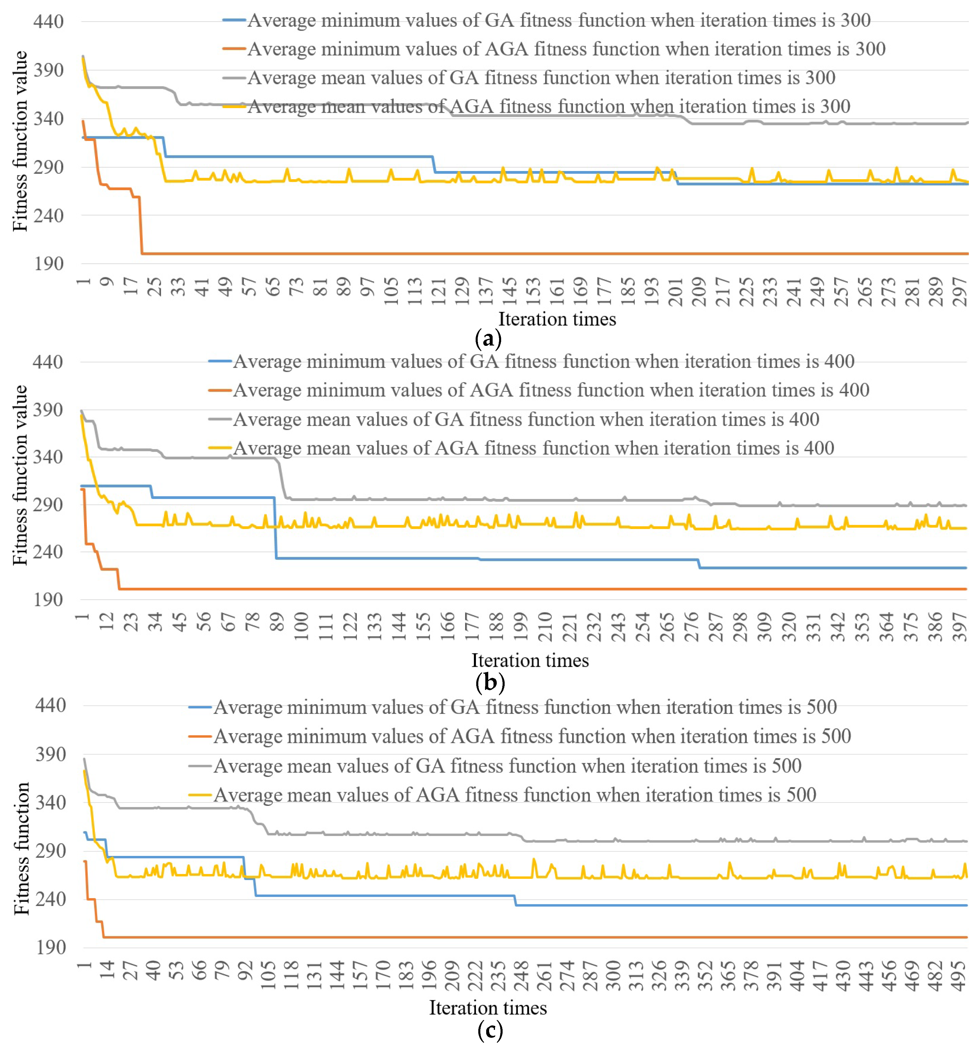
4.1. The Evaluation Experiment of AGA
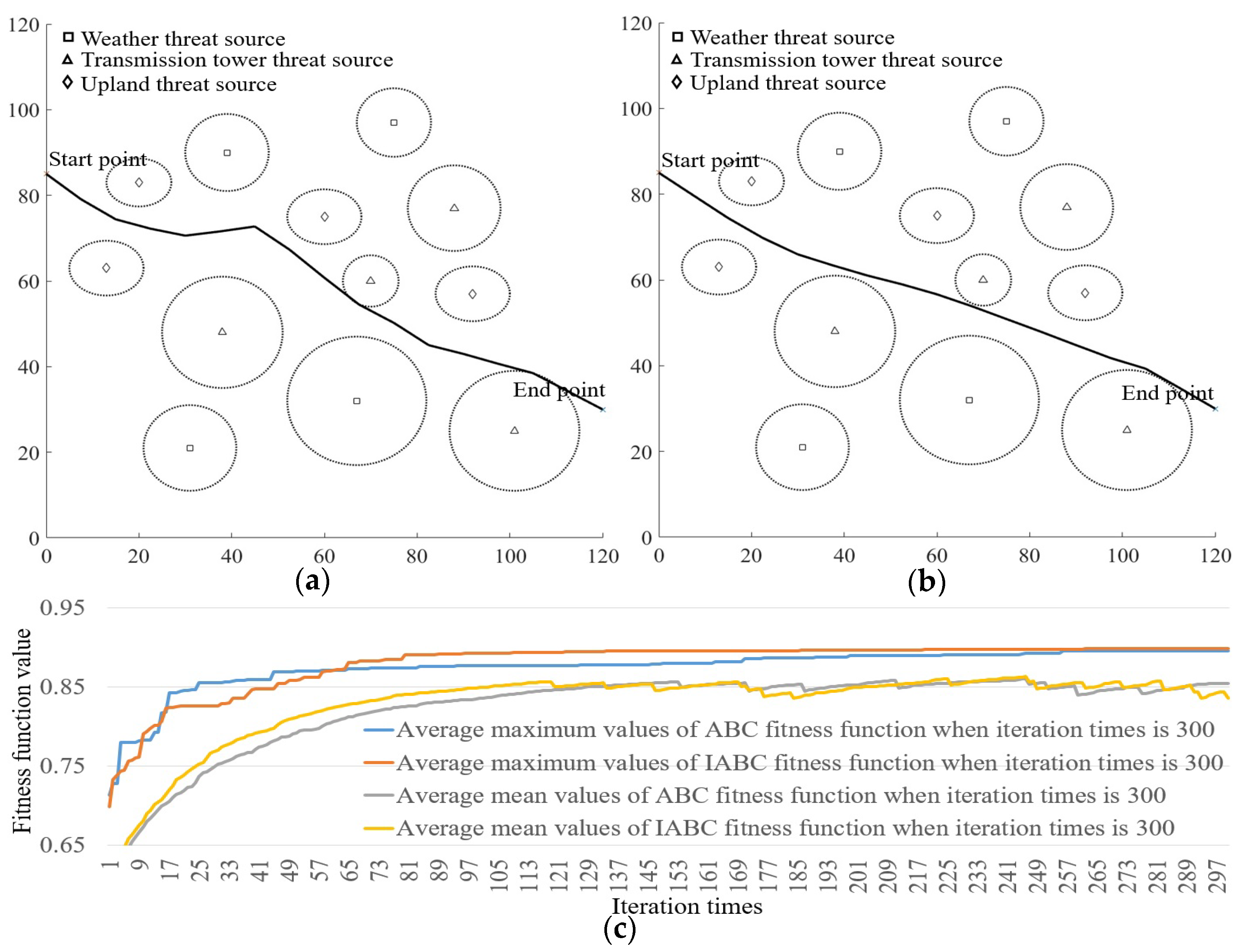
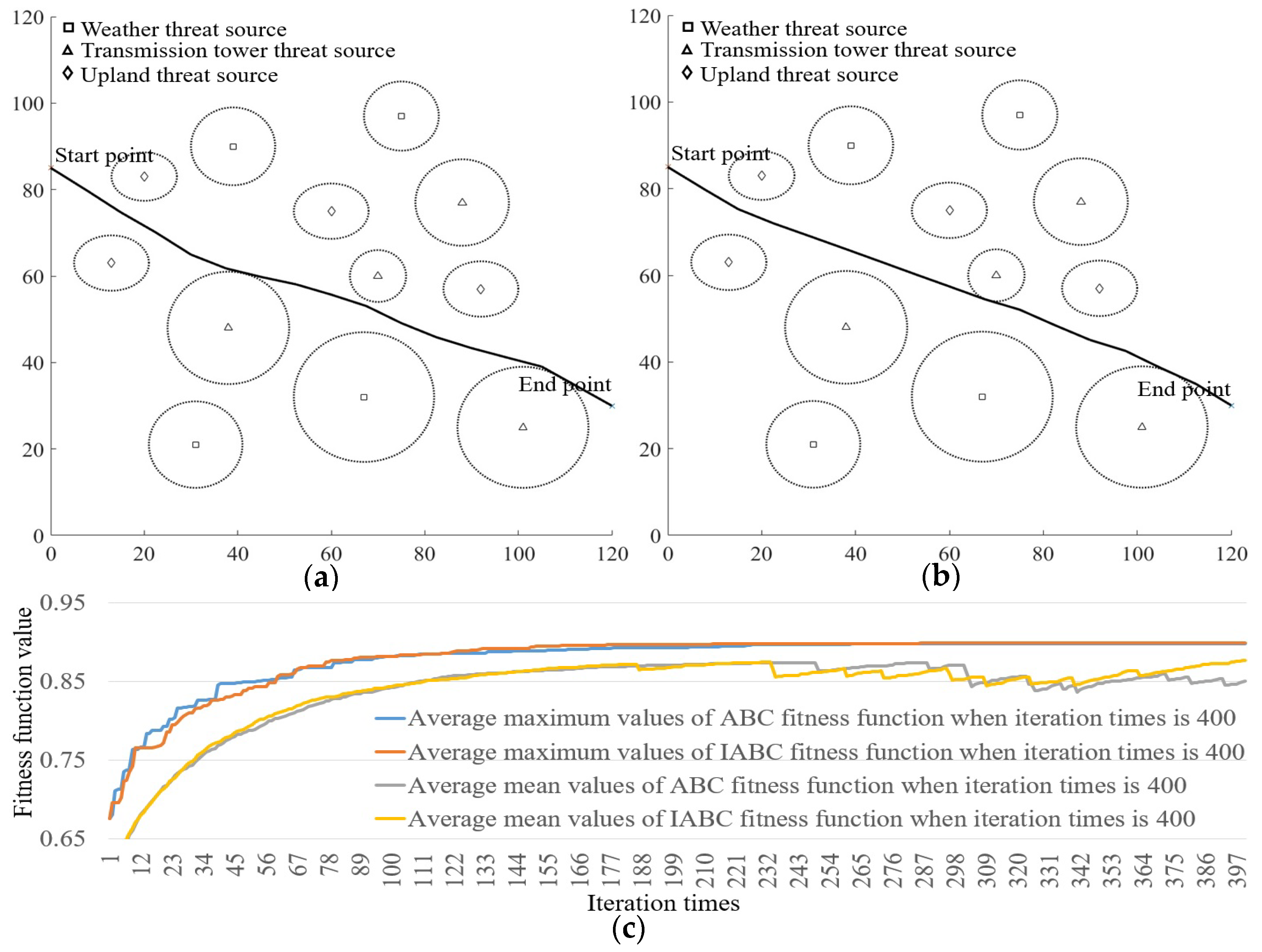
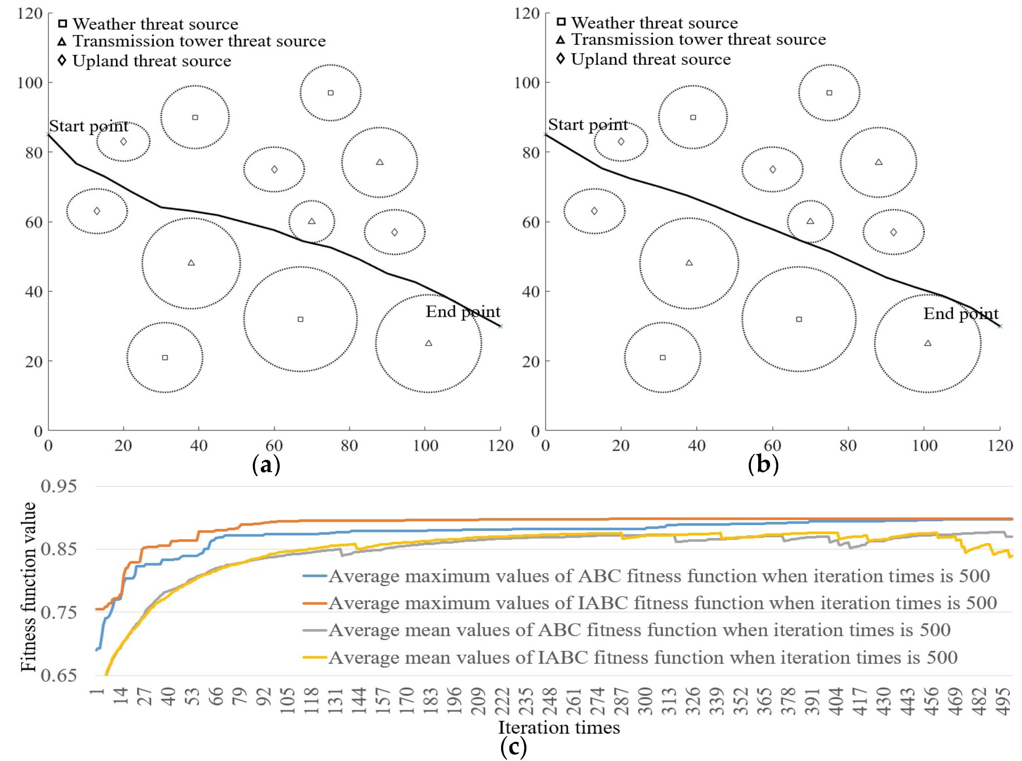
4.2. The Evaluation Experiment of IABC
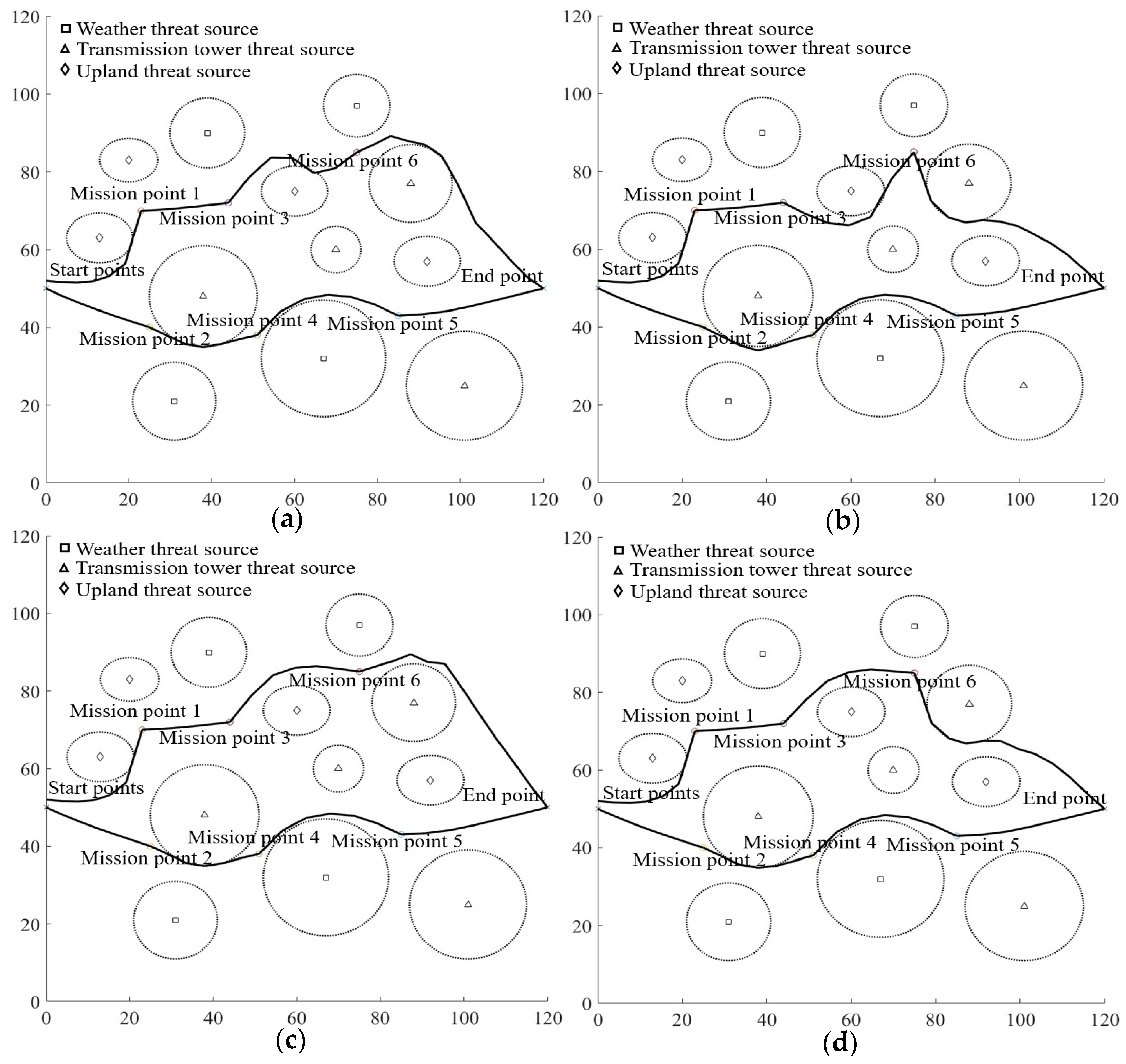
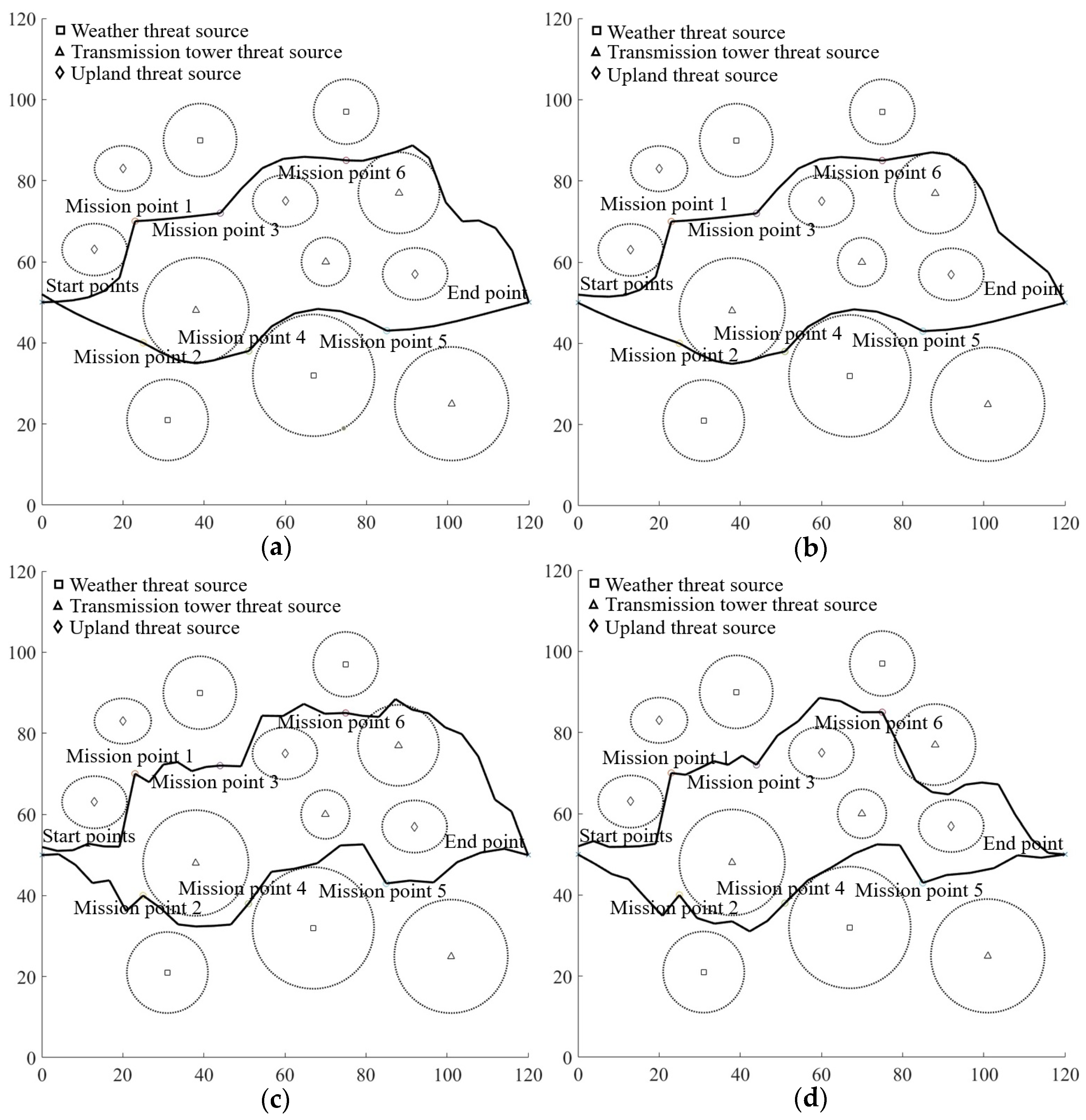
4.3. The Evaluation Experiment of Disaster Rescue Simulation
4.4. Discussions
5. Conclusions
Author Contributions
Funding
Conflicts of Interest
Abbreviations
| ABC | Artificial bee colony |
| AGA | Adaptive Genetic algorithm |
| AHP | Analytic hierarchy process |
| APFA | Artificial potential field algorithm |
| GA | Genetic algorithm |
| GMM | Gaussian mixed model |
| IABC | Improved artificial bee colony |
| LES | Large Eddy Simulations |
| PC | Personal computer |
| PSO | Particle swarm optimization |
| UAV | Unmanned aerial vehicle |
| WRF | Weather research and forecasting |
Nomenclature
| The threat degree of rain and wind of the ith UAV in the jth threat source under the pth iterative computation. | |
| The threat degree of rain of the ith UAV in the jth threat source under the pth iterative computation. | |
| The threat degree of wind of the ith UAV in the jth threat source under the pth iterative computation. | |
| The distance between UAV and weather threat source center. | |
| The radius of weather threat source. | |
| The integrated weather threat degree of the ith UAV under the pth iterative computation. | |
| The total amount of weather threat source. | |
| The probability density function of bi-GMM function of the ith UAV in the jth threat source under the pth iterative computation, q is the number of Gaussian function. | |
| The mean of Gaussian function 1 of the ith UAV in the jth threat source under the pth iterative computation, q is the number of Gaussian function. | |
| The mean of Gaussian function 2 of the ith UAV in the jth threat source under the pth iterative computation, q is the number of Gaussian function. | |
| The variance of Gaussian function 1 of the ith UAV in the jth threat source under the pth iterative computation, q is the number of Gaussian function. | |
| The variance of Gaussian function 2 of the ith UAV in the jth threat source under the pth iterative computation, q is the number of Gaussian function. | |
| The correlation coefficient of bi-GMM of the ith UAV in the jth threat source under the pth iterative computation, q is the number of Gaussian function. | |
| The threat degree of transmission tower of the ith UAV in the jth threat source under the pth iterative computation. | |
| The weight of Gaussian function, j is the number of threat source, p is number of iteration times, q is the number of Gaussian function. | |
| The integrated transmission tower threat degree of the ith UAV in the pth threat source. | |
| The total number of transmission tower in the investigated area. | |
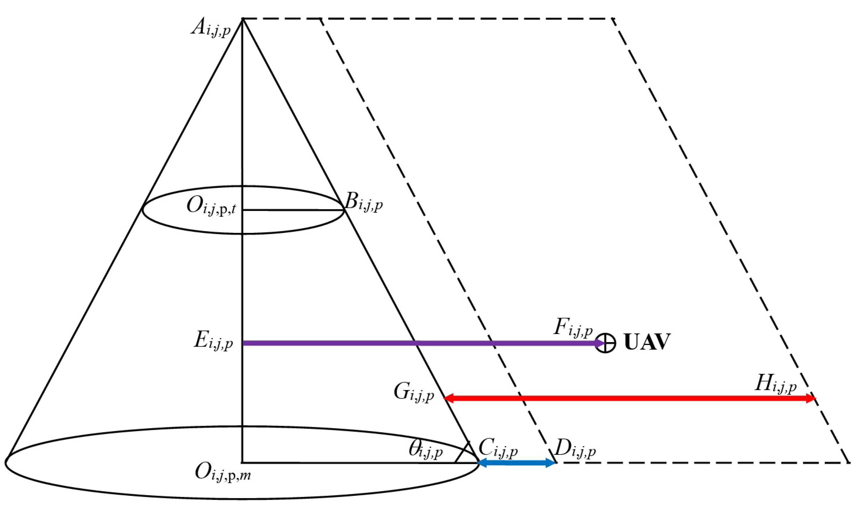
| Please see the definition in Figure 5. | |
| Please see the definition in Figure 5. | |
| Please see the definition in Figure 5. | |
| Please see the definition in Figure 5. | |
| Please see the definition in Figure 5. | |
| Please see the definition in Figure 5. | |
| Please see the definition in Figure 5. | |
| Please see the definition in Figure 5. | |
| The threat degree of upland of the ith UAV in the jth threat source under the pth iterative computation. | |
| The integrated threat degree of upland of the ith UAV under the pth iterative computation. | |
| The total cost and revenue of the ith UAV in the pth iterative computation. | |
| The mission point cost function of the ith UAV under the pth iterative computation. | |
| The recovery point cost function of the ith UAV under the pth iterative computation. | |
| The weight of distance factor of mission point. | |
| The weight of oil consumption factor of mission point. | |
| The weight of weather threat factor of mission point. | |
| The weight of transmission tower threat factor of mission point. | |
| The weight of upland threat factor of mission point. | |
| The total number of mission point. | |
| The weight of distance factor of recovery point. | |
| The weight of oil consumption factor of recovery point. | |
| The weight of weather threat factor of recovery point. | |
| The weight of transmission tower threat factor of recovery point. | |
| The weight of upland threat factor of recovery point. | |
| The distance cost value of mission point k of the ith UAV under the pth iterative computation. | |
| The oil consumption cost value of mission point k of the ith UAV under the pth iterative computation. | |
| The weather cost value of mission point k of the ith UAV under the pth iterative computation. | |
| The transmission tower cost value of mission point k of the ith UAV under the pth iterative computation. | |
| The upland cost value of mission point k of the ith UAV under the pth iterative computation. | |
| The distance cost value of recovery point c of the ith UAV under the pth iterative computation. | |
| The oil consumption cost value of recovery point c of the ith UAV under the pth iterative computation. | |
| The weather cost value of recovery point c of the ith UAV under the pth iterative computation. | |
| The transmission tower cost value of recovery point c of the ith UAV under the pth iterative computation. | |
| The upland cost value of recovery point c of the ith UAV under the pth iterative computation. | |
| The amount of drug delivery UAV under the pth iterative computation. | |
| The amount of image collection UAV under the pth iterative computation. | |
| The amount of communication relay UAV under the pth iterative computation. | |
| The rate of successful drug delivery of drug delivery UAV. | |
| The improvement probability of drug delivery caused by image collection UAV. | |
| The decreasing probability of threat source caused by communication relay UAV. | |
| The revenue of the kth mission point. | |
| The weight of Gaussian function 1. | |
| The weight of Gaussian function 2. | |
| The total amount of UAV. | |
| The fitness function of AGA under the p_AGAth iteration. | |
| The AGA application of Equation (15). | |
| The selection probability of AGA under the p_AGAth iteration. | |
| The maximum population amount of AGA. | |
| The cross probability of AGA under the p_AGAth iteration. | |
| A control parameter of AGA fitness function under the p_AGAth iteration. | |
| A control parameter of AGA fitness function under the p_AGAth iteration. | |
| A control parameter of AGA fitness function under the p_AGAth iteration. | |
| A control parameter of AGA fitness function under the p_AGAth iteration. | |
| The maximum of cross probability of AGA under the p_AGAth iteration. | |
| The maximum of fitness function of AGA under the p_AGAth iteration. | |
| The mean of fitness function of AGA under the p_AGAth iteration. | |
| The mutation probability of AGA under the p_AGAth iteration. | |
| The maximum of mutation probability of AGA under the p_AGAth iteration. | |
| The adjustment parameter of fitness function of AGA. | |
| The iteration times-related variable of AGA algorithm. | |
| The maximum of cost-revenue function under the p_AGAth iteration. | |
| The maximum iteration number of AGA. | |
| The coordinate of flight path. | |
| The minimum value of xij. | |
| The maximum value of xij. | |
| The total amount of bee of ABC algorithm. | |
| The parameter dimension of ABC algorithm. | |
| The fitness function of IABC algorithm. | |
| The cost-revenue function of IABC algorithm under p_IABCth iteration. | |
| The jth dimension component of global optimal solution of current population. | |
| The balanced searching factor 1 of IABC algorithm. | |
| The balanced searching factor 2 of IABC algorithm. | |
| The current iteration number of IABC algorithm. | |
| The maximum iteration number of IABC algorithm. |
References
- Liu, H.; Yan, B.; Wang, W.; Li, X.; Guo, Z. Manhole cover detection from natural scene based on imaging environment perception. KSII Trans. Internet Inf. 2019, 13, 5059–5111. [Google Scholar]
- Lv, M.; Zheng, J.; Tong, Q.; Chen, J.; Liu, H.; Gao, Y. Modeling and simulation of scheduling medical materials using graph model for complex rescue. J. Inf. Process. Syst. 2017, 13, 1243–1258. [Google Scholar]
- Chen, J.; Liu, H.; Zheng, J.; Lv, M.; Yan, B.; Hu, X.; Gao, Y. Damage degree evaluation of earthquake area using UAV aerial image. Int. J. Aerosp. Eng. 2016, 216, 2052603. [Google Scholar] [CrossRef] [Green Version]
- Liu, H.; Wang, W.; He, Z.; Tong, Q.; Wang, X.; Yu, W.; Lv, M. The design of air-space integrative calamity information analysis and rescue system. In Proceedings of the IEEE International Conference on Cyber Technology in Automation, Control and Intelligent Systems, Shenyang, China, 8–12 June 2015; pp. 1997–2001. [Google Scholar]
- Yamazaki, F.; Miyazaki, S.; Liu, W. 3D visualization of landslide affected area due to heavy rainfall in Japan from UAV flights and SfM. In Proceedings of the IEEE International Geoscience and Remote Sensing Symposium, Valencia, Spain, 22–27 July 2018; pp. 5685–5688. [Google Scholar]
- Fan, Q.; Wang, F.; Shen, X.; Luo, D. Path planning for a reconnaissance UAV uncertain environment. In Proceedings of the IEEE International Conference on Control and Automation, Kathmandu, Nepal, 1–3 June 2016; pp. 248–252. [Google Scholar]
- Hao, R.; Luo, D.; Duan, H. Multiple UAVs mission assignment based on modified pigeon-inspired optimization algorithm. In Proceedings of the IEEE Chinese Guidance, Navigation and Control Conference, Yantai, China, 8–10 August 2014; pp. 2692–2697. [Google Scholar]
- He, Z.; Zhao, L. The comparison of four UAV path planning algorithms based on geometry search algorithm. In Proceedings of the International Conference on Intelligent Human-Machine Systems and Cybernetics, Hangzhou, China, 26–27 August 2017; pp. 33–36. [Google Scholar]
- Cichella, V.; Kaminer, I.; Dobrokhodov, V.; Xargay, E.; Choe, R.; Hovakimyan, N.; Pedro Aguiar, A.; Pascoal, A.M. Cooperative path following of multiple multirotors over time-varying networks. IEEE Trans. Autom. Sci. Eng. 2015, 12, 945–957. [Google Scholar] [CrossRef]
- Oh, H.; Turchi, D.; Kim, S.; Tsourdos, A.; Pollini, L.; White, B. Coordinated standoff tracking using path sha** for multiple UAVs. IEEE Trans. Aerosp. Electron. Syst. 2014, 50, 348–363. [Google Scholar] [CrossRef] [Green Version]
- Nguyen, H.V.; Rezatofighi, H.; Vo, B.-N.; Ranasinghe, D.C. Online UAV path planning for joint detection and tracking of multiple radio-tagged objects. IEEE Trans. Signal Process. 2019, 67, 5365–5379. [Google Scholar] [CrossRef] [Green Version]
- ** for precision farming. IEEE Robot. Autom. Lett. 2019, 4, 1086–1092. [Google Scholar] [CrossRef] [Green Version]
- Rezinkina, M.; Rezinkin, O.; Lytvynenko, S.; Tomashevskyi, R. Electromagnetic compatibility at UAVs usage for power transmission lines monitoring. In Proceedings of the IEEE International Conference Actual Problems of Unmanned Aerial Vehicles Developments, Kiev, Ukraine, 22–24 October 2019; pp. 157–160. [Google Scholar]


| Representative Algorithm | Algorithm Category | |||
| Heuristic Algorithm | Mathematical Programming | Stochastic Intelligent Optimization Method | ||
| Mission assignment problem | Tabu search algorithm [13], simulated annealing algorithm [14], genetic algorithm (GA) [15], etc. | Enumeration algorithm [16], dynamic programming [17], etc. | Evolutionary computation [18], swarm intelligence computing [19], artificial immune algorithm [20], etc. | |
| Representative Algorithm | Algorithm Category | |||
| Mathematical Programming | Artificial Potential Field Method | Graph-Based Method | Intelligent Optimization Method | |
| Path planning problem | Dynamic programming [21], nonlinear programming method [22], etc. | Basic artificial potential field method [23], improved artificial potential field method [24], etc. | Dijkstra algorithm [25], A* algorithm [26], Voronoi diagram method [27], probabilistic roadmaps method [28], etc. | Swarm intelligence computing [29], bionic algorithm [30], etc. |
| Wind Speed (m/s) | (0.0, 0.2] | (0.2, 7.9] | (7.9, 13.8] | (13.8, 24.4] | (24.4, 100.0] |
| Threat Degree | 1 | 2 | 3 | 4 | 5 |
| Intensity of Importance | Definition |
|---|---|
| 1 | Equally important |
| 3 | Weakly important |
| 5 | Essentially important |
| 7 | Very strongly important |
| 9 | Absolutely important |
| 2, 4, 6, 8 | Importance between the above odd numbers |
| Test Experiment 1 | |||
| Number of Mission Point | Coordinate of Mission Point | Number of Mission Point | Coordinate of Mission Point |
| 1 | (50, 70) | 5 | (75, 75) |
| 2 | (20, 48) | 6 | (90, 30) |
| 3 | (30, 65) | 7 | (26, 30) |
| 4 | (60, 80) | 8 | (80, 40) |
| Test Experiment 2 | |||
| Number of Mission Point | Coordinate of Mission Point | Number of Mission Point | Coordinate of Mission Point |
| 1 | (50, 70) | 10 | (105, 60) |
| 2 | (20, 48) | 11 | (98, 49) |
| 3 | (30, 65) | 12 | (93, 87) |
| 4 | (60, 80) | 13 | (47, 12) |
| 5 | (75, 75) | 14 | (84, 17) |
| 6 | (90, 30) | 15 | (39, 75) |
| 7 | (26, 30) | 16 | (98, 74) |
| 8 | (80, 40) | 17 | (75, 24) |
| 9 | (60, 20) | 18 | (39, 8) |
| Fitness Function Value | |||||
| Best Value | Worst Value | Standard Deviation Value | Mean Value | ||
| Test experiment 1 | GA | 203.5649 | 322.9047 | 33.6182 | 261.5839 |
| AGA | 200.8118 | 286.4434 | 30.7327 | 225.2601 | |
| Text experiment 2 | GA | 506.3372 | 744.7273 | 56.8380 | 623.5432 |
| AGA | 369.5323 | 493.2025 | 30.5143 | 429.6063 | |
| Processing Time (s) | |||||
| Best Value | Worst Value | Standard Deviation Value | Mean Value | ||
| Test experiment 1 | GA | 1.61 | 2.16 | 0.11 | 1.75 |
| AGA | 1.92 | 2.75 | 0.24 | 2.49 | |
| Text experiment 2 | GA | 2.1 | 3.1 | 0.26 | 2.59 |
| AGA | 3.36 | 4.44 | 0.16 | 3.86 | |
| Result of Optimal Mission Point Schedule | ||||
|---|---|---|---|---|
| Iteration Times = 300 | Iteration Times = 400 | Iteration Times = 500 | ||
| Test experiment 1 | GA | 2, 3, 4, 5, 1, 7, 6, 8 | 2, 7, 3, 1, 5, 4, 8, 6 | 7, 3, 2, 1, 4, 5, 8, 6 |
| AGA | 7, 2, 3, 1, 4, 5, 8, 6 | 7, 2, 3, 1, 4, 5, 8, 6 | 7, 2, 3, 1, 4, 5, 8,6 | |
| Test experiment 2 | GA | 13, 8, 6, 4, 5, 11, 10, 12, 16, 17, 9, 2, 1, 15, 3, 18, 7, 14 | 14, 9, 13, 2, 1, 11, 10, 16, 17, 18, 7, 15, 3, 4, 5, 12, 8, 6 | 7, 2, 14, 6, 10, 11, 8, 17, 9, 13, 18, 16, 12, 15, 1, 3, 4, 5 |
| AGA | 2, 1, 12, 16, 10, 11, 17, 14, 6, 8, 5, 4, 15, 3, 7, 18, 13, 9 | 13, 18, 7, 2, 3, 15, 1, 9, 14, 17, 4, 5, 12, 16, 8, 6, 11, 10 | 3, 15, 1, 17, 9, 2, 7, 18, 13, 14, 6, 8, 11, 5, 4, 12, 16, 10 | |
| Num | Center Coordinate, Radius, Rain State a, and Wind Degree of Severe Weather Threat Source | Center Coordinate, (μ1i,j, p,1, σ12i,j,p,1), (μ2i,j,p.2, σ22i,j,p.2), wj,p,1, and wj,p.2 of Transmission Tower Threat Source | Center Coordinate, Minimum Height, Maximum Height, and Radius of Upland Threat Source |
|---|---|---|---|
| 1 | (31, 21), 10, 0, 4 | (13, 63), (1, 5), (1, 9), 0.5, 0.5 | (38, 48), 150, 300, 13 |
| 2 | (67, 32), 15, 1, 2 | (60, 75), (2, 6), (2, 10), 0.5, 0.5 | (88, 77), 150, 300, 10 |
| 3 | (75, 97), 8, 0, 3 | (20, 83), (3, 7), (3,11), 0.5, 0.5 | (70, 60), 150, 300, 6 |
| 4 | (39, 90), 9, 0, 3 | (92, 57), (4, 8), (4, 12), 0.5, 0.5 | (101, 25), 150, 300, 14 |
| Iteration Times | Method | Optimal Fitness Function | Path Length | Processing Time |
| 300 | ABC | 0.8957 | 172.5320 | 3.58 |
| IABC | 0.8984 | 167.8581 | 5.76 | |
| Iteration Times | Method | Optimal Fitness Function | Path Length | Processing Time |
| 400 | ABC | 0.8980 | 168.1855 | 4.51 |
| IABC | 0.8987 | 167.7283 | 7.42 | |
| Iteration Times | Method | Optimal Fitness Function | Path Length | Processing Time |
| 500 | ABC | 0.8975 | 167.4791 | 5.54 |
| IABC | 0.8987 | 167.4733 | 9.03 |
| Fitness Function/The Iteration Times Is 300 | ||||
| Best Value | Worst Value | Standard Deviation Value | Mean Value | |
| ABC | 0.8985 | 0.8943 | 1.3 × 10⁻³ | 0.8972 |
| IACB | 0.8986 | 0.8967 | 4.6143 × 10⁻⁴ | 0.8981 |
| Path Length/The Iteration Times Is 300 | ||||
| Best Value | Worst Value | Standard Deviation Value | Mean Value | |
| ABC | 167.2298 | 172.5320 | 1.3489 | 168.6910 |
| IACB | 164.8105 | 168.5795 | 0.97294 | 167.6903 |
| Processing Time (s)/The Iteration Times Is 300 | ||||
| Best Value | Worst Value | Standard Deviation Value | Mean Value | |
| ABC | 3.56 | 4.27 | 0.1541 | 3.95 |
| IACB | 5.70 | 6.36 | 0.1322 | 6.02 |
| Fitness Function/The Iteration Times Is 400 | ||||
| Best Value | Worst Value | Standard Deviation Value | Mean Value | |
| ABC | 0.8987 | 0.8964 | 5.3594 × 10⁻⁴ | 0.8982 |
| IACB | 0.8988 | 0.8981 | 1.7287 × 10⁻⁴ | 0.8986 |
| Path Length/The Iteration Times is 400 | ||||
| Best Value | Worst Value | Standard Deviation Value | Mean Value | |
| ABC | 166.6625 | 169.4589 | 0.6558 | 168.2398 |
| IACB | 166.5989 | 168.4041 | 0.4691 | 167.8869 |
| Processing Time (s)/The Iteration Times Is 400 | ||||
| Best Value | Worst Value | Standard Deviation Value | Mean Value | |
| ABC | 5.23 | 4.53 | 0.1462 | 4.70 |
| IACB | 7.86 | 7.55 | 0.0778 | 7.68 |
| Fitness Function/The Iteration Times Is 500 | ||||
| Best Value | Worst Value | Standard Deviation Value | Mean Value | |
| ABC | 0.8987 | 0.8975 | 2.8031 × 10⁻⁴ | 0.8985 |
| IACB | 0.8988 | 0.8982 | 1.3235 × 10⁻⁴ | 0.8987 |
| Path Length/The Iteration Times is 500 | ||||
| Best Value | Worst Value | Standard Deviation Value | Mean Value | |
| ABC | 167.4791 | 169.0534 | 0.3398 | 168.4406 |
| IACB | 167.3409 | 168.5107 | 0.2934 | 168.2355 |
| Processing Time (s)/The Iteration Times Is 500 | ||||
| Best Value | Worst Value | Standard Deviation Value | Mean Value | |
| ABC | 5.29 | 6.09 | 0.2080 | 5.60 |
| IACB | 8.83 | 10.13 | 0.3193 | 9.41 |
| Threat Source | UAV Performance | |
|---|---|---|
| Threat source | 1 | 7 |
| UAV performance | 1/7 | 1 |
| Oil consumption () | 1 | 9 |
| Flight distance () | 1/9 | 1 |
| Weather () | 1 | 9 | 9 |
| Transmission tower () | 1/9 | 1 | 1 |
| Upland () | 1/9 | 1 | 1 |
| Name | |||||
| Value | 0.0125 | 0.1125 | 0.7159 | 0.0795 | 0.0795 |
| Threat Source | UAV Performance | |
|---|---|---|
| Threat source | 1 | 3 |
| UAV performance | 1/3 | 1 |
| Flight Distance () | ||
|---|---|---|
| Oil consumption () | 1 | 6 |
| Flight distance () | 1/6 | 1 |
| Weather () | 1 | 8 | 8 |
| Transmission tower () | 1/8 | 1 | 2 |
| Upland () | 1/8 | 1/2 | 1 |
| Name | |||||
| Value | 0.2143 | 0.0357 | 0.5968 | 0.094 | 0.0592 |
| Number of Mission Point | Coordinate of Mission Point | Number of Mission Point | Coordinate of Mission Point | Number of Mission Point | Coordinate of Mission Point |
|---|---|---|---|---|---|
| 1 | (23, 70) | 3 | (44, 72) | 5 | (85, 43) |
| 2 | (25, 40) | 4 | (51, 38) | 6 | (75, 82) |
| Method Name | Group Assignment Result a | Mission Assignment Result b | Total Revenue Result | Total Cost Result | Processing Time (s) | Path Length |
|---|---|---|---|---|---|---|
| GA+ABC | Group A: 8, 1, 2 Group B: 7, 2, 0 | Group A: 1, 3, 6 Group B: 2, 4, 5 | 79.5684 | 0.1453 | 62.27 | 340.9001 |
| GA+IABC | Group A: 7, 2, 0 Group B: 8, 1, 2 | Group A: 2, 4, 5 Group B: 1, 3, 6 | 79.4320 | 0.1633 | 82.44 | 334.9619 |
| AGA+ABC | Group A: 7, 2, 0 Group B: 8, 1, 2 | Group A: 2, 4, 5 Group B: 1, 3, 6 | 79.5740 | 0.1435 | 92.62 | 337.5118 |
| AGA+IABC | Group A: 7, 2, 0 Group B: 8, 1, 2 | Group A: 2, 4, 5 Group B: 1, 3, 6 | 79.6475 | 0.1326 | 113.68 | 329.1168 |
| Average Revenue Result | ||||
| Best Value | Worst Value | Standard Deviation Value | Mean Value | |
| GA+ABC | 79.6017 | 79.1356 | 0.1157 | 79.4761 |
| GA+IABC | 79.6265 | 79.3540 | 0.0706 | 79.5123 |
| AGA+ABC | 79.5799 | 77.7220 | 0.5315 | 79.3207 |
| AGA+IABC | 79.6475 | 79.4919 | 0.0363 | 79.5749 |
| Average Cost Result | ||||
| Best Value | Worst Value | Standard Deviation Value | Mean Value | |
| GA+ABC | 0.1418 | 0.1788 | 0.0105 | 0.1534 |
| GA+IABC | 0.1350 | 0.1633 | 0.0072 | 0.1461 |
| AGA+ABC | 0.1374 | 0.1985 | 0.0174 | 0.1530 |
| AGA+IABC | 0.1326 | 0.1489 | 0.0039 | 0.1413 |
| Average Processing Time (s) | ||||
| Best Value | Worst Value | Standard Deviation Value | Mean Value | |
| GA+ABC | 61.31 | 69.34 | 2.1148 | 64.52 |
| GA+IABC | 79.13 | 86.84 | 2.1571 | 83.54 |
| AGA+ABC | 89.92 | 95.73 | 1.9324 | 93.08 |
| AGA+IABC | 102.24 | 114.87 | 3.4733 | 108.71 |
| Average Path Length | ||||
| Best Value | Worst Value | Standard Deviation Value | Mean Value | |
| GA+ABC | 329.5748 | 340.9091 | 3.7418 | 336.6497 |
| GA+IABC | 329.8217 | 343.4356 | 3.4055 | 334.4394 |
| AGA+ABC | 331.0667 | 379.0624 | 12.5883 | 339.6279 |
| AGA+IABC | 328.6109 | 337.5947 | 2.7720 | 331.9636 |
| Average Revenue Result | ||||
| Best Value | Worst Value | Standard Deviation Value | Mean Value | |
| GA+PSO | 79.5746 | 77.4224 | 0.7295 | 79.0008 |
| AGA+PSO | 79.5918 | 78.0337 | 0.3909 | 79.3464 |
| GA+APFA | 79.4929 | 77.5304 | 0.5118 | 79.0061 |
| AGA+APFA | 79.5426 | 78.9268 | 0.1757 | 79.3605 |
| Average Cost Result | ||||
| Best Value | Worst Value | Standard Deviation Value | Mean Value | |
| GA+PSO | 0.1444 | 0.2815 | 0.0317 | 0.1615 |
| AGA+PSO | 0.1411 | 0.1919 | 0.0170 | 0.1533 |
| GA+APFA | 0.1445 | 0.1847 | 0.0116 | 0.1601 |
| AGA+APFA | 0.1419 | 0.1721 | 0.0083 | 0.1508 |
| Average Processing Time (s) | ||||
| Best Value | Worst Value | Standard Deviation Value | Mean Value | |
| GA+PSO | 112.47 | 120.24 | 115.82 | 2.8234 |
| AGA+PSO | 178.92 | 188.56 | 185.02 | 1.8648 |
| GA+APFA | 1694.52 | 1798.42 | 30.5664 | 1740.98 |
| AGA+APFA | 1802.07 | 1892.88 | 25.0210 | 1855.64 |
| Average Path Length | ||||
| Best Value | Worst Value | Standard deviation Value | Mean Value | |
| GA+PSO | 329.8403 | 397.2150 | 19.3590 | 352.9970 |
| AGA+PSO | 330.4529 | 344.4585 | 14.9107 | 350.3686 |
| GA+APFA | 364.3596 | 432.0467 | 16.3501 | 379.0128 |
| AGA+APFA | 358.4359 | 379.2276 | 6.5640 | 367.8603 |
Publisher’s Note: MDPI stays neutral with regard to jurisdictional claims in published maps and institutional affiliations. |
© 2021 by the authors. Licensee MDPI, Basel, Switzerland. This article is an open access article distributed under the terms and conditions of the Creative Commons Attribution (CC BY) license (https://creativecommons.org/licenses/by/4.0/).
Share and Cite
Liu, H.; Ge, J.; Wang, Y.; Li, J.; Ding, K.; Zhang, Z.; Guo, Z.; Li, W.; Lan, J. Multi-UAV Optimal Mission Assignment and Path Planning for Disaster Rescue Using Adaptive Genetic Algorithm and Improved Artificial Bee Colony Method. Actuators 2022, 11, 4. https://doi.org/10.3390/act11010004
Liu H, Ge J, Wang Y, Li J, Ding K, Zhang Z, Guo Z, Li W, Lan J. Multi-UAV Optimal Mission Assignment and Path Planning for Disaster Rescue Using Adaptive Genetic Algorithm and Improved Artificial Bee Colony Method. Actuators. 2022; 11(1):4. https://doi.org/10.3390/act11010004
Chicago/Turabian StyleLiu, Haoting, Jianyue Ge, Yuan Wang, Jiacheng Li, Kai Ding, Zhiqiang Zhang, Zhenhui Guo, Wei Li, and **hui Lan. 2022. "Multi-UAV Optimal Mission Assignment and Path Planning for Disaster Rescue Using Adaptive Genetic Algorithm and Improved Artificial Bee Colony Method" Actuators 11, no. 1: 4. https://doi.org/10.3390/act11010004