1. Introduction
Aircraft type recognition is critical in both civil and military applications because it is a necessary component of target recognition in remote sensing images. However, the task is extremely difficult because of the existence of fine-grained features, which can cause small inter-class changes due to highly comparable subcategories and large intra-class changes due to variances in size, posture, and angle. For instance,
Figure 1 illustrates three types of transport aircraft in series, namely, the C-5, C-17, and C-130. Although these aircraft have distinct purposes and roles, they are visually similar.
Numerous methods have been suggested for aircraft type identification, and they may be classified into three categories: deep-neural-network-based methods [
1,
2,
3,
4,
5], template-matching-based methods [
1,
3,
6], and handcrafted-feature-based methods [
7,
8,
9].
The template-matching-based method involves constructing a template through image segmentation and key point extraction and then making similarity judgments by using the new image. For example, Wu et al. [
6] presented a similarity measure based on reconstruction, which transforms the problem of type identification into one of reconstruction. Subsequently, the authors used a jigsaw reconstruction approach to solve the reconstruction problem to match the result with the standard template. To recognize airplanes, Zhao et al. [
1] converted the aircraft identification problem into a landmark detection problem and used keypoint template matching. Furthermore, to provide accurate and comprehensive representations of airplanes, Zuo et al. [
3] developed an aircraft segmentation network and a keypoint detection network. Next, they performed template matching to recognize aircraft types. However, the template matching method is affected by the target attitude, weather, and other factors, and it cannot be used to accurately extract aircraft shapes in complex scenes [
2].
Based on the method for the recognition of handcrafted features, aircraft images are extracted by using artificially designed features such as the scale-invariant feature transform (SIFT). Ref. [
10] and histogram of oriented gradients (HOG) [
11], and the extracted features are sent to a classifier such as SVM for classification and discrimination.For instance, by using several modular neural network classifiers, Rong et al. [
7] recognized different types of aircraft. Three moment invariants, namely the wavelet moment, Zernike moment, and Hu moment, were derived from the airplane characteristics and utilized as the input variables for each modular neural network. Hsieh et al. [
8] suggested a method based on the hierarchical classification of four distinct characteristics, namely the bitmap, wavelet transformation, distance transformation, and Zernike moment. However, with the use of artificially designed features, it is difficult to accurately describe prior knowledge of the target, and feature generalization is less robust and generalizable [
4].
Recently, deep neural networks have been extensively used in a variety of areas, including classification [
12,
13,
14], detection [
15,
16], object tracking [
17,
18,
19,
20,
21], and segmentation [
22,
23], due to their capacity to learn robust features independently. Deep neural networks, in particular, have facilitated advances in aircraft recognition in remote sensing images. For instance, Diao et al. [
4] presented a novel pixel-wise learning approach for object recognition based on deep belief networks. Zhao et al. [
1] proposed an aircraft landmark detection method to address aircraft type recognition. This method detects the landmark points of an aircraft by using a vanilla network. Zuo et al. [
3] adopted a convolutional neural network (CNN)-based image segmentation method to extract the keypoints of an aircraft object and later implemented template matching to perform object recognition. Zhang et al. [
5] presented a conditional generative adversarial network (GAN)-based aircraft type recognition system. Without type labels, the proposed system can learn representative characteristics from images. To extract the discriminative portions of airplanes of various categories, Fu et al. [
2] developed a multiple-class activation map** method.
Compared to handcrafted feature-based machine learning, neural network-based models exhibit significant gains in terms of generalization and robustness. However, these models have the following limitations: (1) the backpropagation (BP) algorithm must be used to perform iterative optimization, meaning that the training process is time-intensive. (2) A considerable volume of training data is required to maintain an elevated level of performance. However, collecting aircraft model samples is a challenging task. Hence, the sample size is often excessively small to support deep neural networks in training, and the resulting models tend to suffer from overfitting. (3) Deep neural network training requires significant computing and storage resources and cannot be effectively implemented in certain resource-constrained environments.
By contrast, shallow feature learning algorithms require fewer computational resources, and their performance is comparable to that of neural-network-based models in certain tasks. For example, Chan et al. [
24] suggested a straightforward deep learning network for image recognition, which was composed entirely of the most fundamental data-processing components: block-wise histograms, binary hashing, and principal component analysis.
The extreme learning machine (ELM) [
25] is a straightforward and extremely powerful feedforward network with a single hidden layer (SLFN). In comparison to standard SLFN training methods, the ELM can attain significantly higher training speeds while allowing for universal approximation [
26]. These aspects can be attributed to the use of fixed hidden neurons and tunable output weights. The ELM can be used to accomplish a variety of tasks, including data representation learning [
27,
28,
29] and classification [
30]. Huang et al. [
27] suggested an object recognition method based on the local-receptive-field-based extreme learning machine (ELM-LRF), which is often used to manage raw images directly. The framework generates random weights for the input and analytically calculates the output weights, which leads to a simple and deterministic solution. Zhu et al. [
28] presented hierarchical neural networks based on an ELM autoencoder (ELM-AE) [
29] to promptly learn local receptive filters and achieve trans-layer representation. Zong et al. [
30] presented a weighted ELM to address data with an imbalanced class distribution.
To enhance the efficiency of the existing machine learning models, researchers have focused on facilitating learning by considering the local consistency of data. Peng et al. proposed a discriminative graph-regularized ELM (GELM) [
31]. The GELM combines the discriminant information of multiple data samples to construct a Laplacian eigenmap (LE) [
32] structure that is incorporated as a regular term in the ELM algorithm. In the generalized ELM autoencoder (GELM-AE) introduced by K. Sun et al. [
33], manifold regularization is performed to restrict the ELM-AE to learn local-geometry-preserving representations. To determine both local geometry and global discriminatory information in the representation space, H. Ge et al. [
34] developed a graph-embedded denoising ELM autoencoder (GDELM-AE) by integrating local Fisher discrimination analysis into the ELM-AE. Inspired by these studies, we incorporate the geometric information of given data into the recognition model to reduce the effect of small intra-class and large inter-class differences on aircraft recognition models.
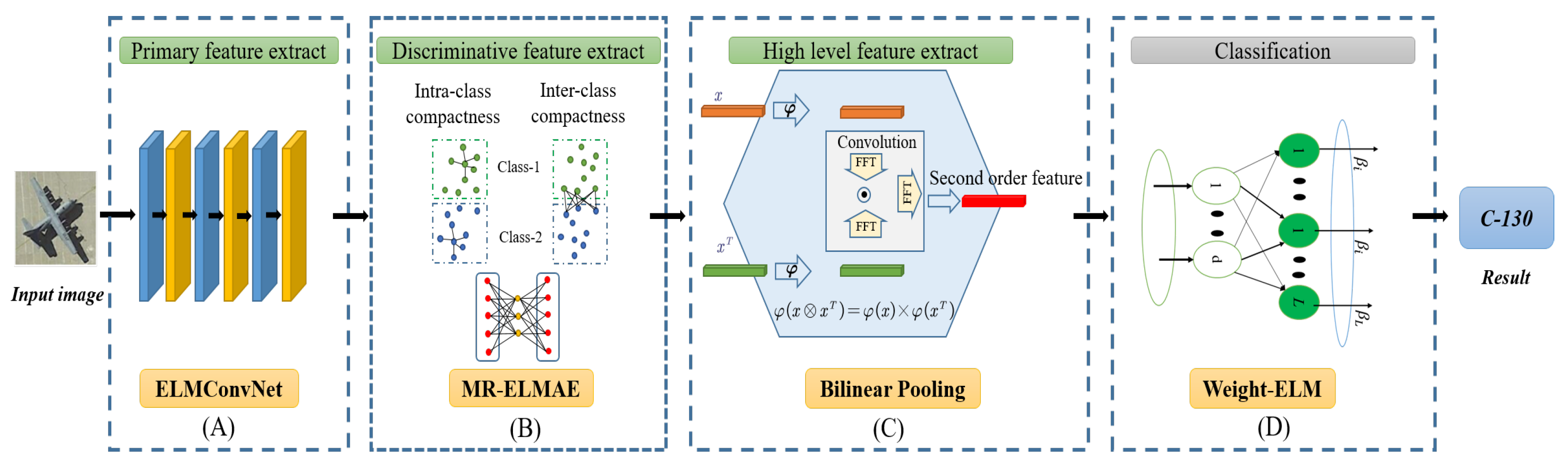
To solve the problems mentioned earlier in this section, we propose a bilinear discriminative ELM network (BD-ELMNet) by drawing on the ideas of the local receptive field ELM, manifold regularization, and bilinear pooling. We optimize the CNN from the viewpoints of the training strategy and feature extraction. As the training strategy, layer-by-layer autoencoder training is performed to train the convolution parameters, which helps us to prevent the consumption of considerable computing resources due to BP and reduce the required sample size. We designed a four-step feature extraction procedure, and the steps are as follows: primary feature extraction, intermediate discriminative feature extraction, high-level feature extraction, and supervised classification. The primary feature extraction module uses the ELMConvNet network, which introduces multiple convolutions and pooling operations based on a single-layer ELM-LRF. To enhance the image classification and processing capabilities, the network structure can extract abstract image information and ensure the invariance of the displacement of data feature attributes. To realize intermediate discriminant feature extraction, a manifold regularized ELM autoencoder (MRELM-AE) is used to extract strong discriminative features, which can learn data representations from the local geometry and local discriminants extracted from the input data by minimizing the intra-class distance and maximizing the inter-class distance. In the MRELM-AE, the constraints imposed on the output weight force the outputs of similar and distinct samples to be close to and far from one another in the new space, respectively. The constraint is a manifold regularization term that is added to the goal of the original ELM-AE model. The output weights may then be solved analytically. In the high-order feature extraction module, the bilinear pool model is used as the high-order feature extractor of the BD-ELMNet, which extracts second-order statistical information by calculating the outer product of the feature description vectors. This second-order statistical information can reflect the correlation between feature dimensions and generate an expressive global representation that can significantly enhance the classification performance of the model. Finally, we employ the weighted ELM as a supervised classifier to alleviate the problem of data imbalance.
The main contributions of this paper can be summarized as follows:
- (1)
We propose a novel aircraft recognition framework that not only inherits the characteristics of the ELM’s training speed but also relies on convolution, MRELM-AE, and bilinear pooling to construct a three-level feature extractor, as a result of which the aircraft recognition model exhibits strong discrimination features.
- (2)
We propose a novel discriminant MRELM-AE, which adds the manifold regularization to the objective of the ELM-AE. The manifold regularization considers the geometric structure and distinguishing information of the data to enhance the feature expression ability of the ELM-AE.
- (3)
The experimental results on the MTARSI dataset [
35] show that the BD-ELMNet outperforms the state-of-the-art deep learning method in terms of its training speed and accuracy.
The remainder of this article is organized as follows. In
Section 2, we briefly introduce the works related to convolutional neural networks, pooling methods, data augmentation techniques and discriminative ELM. In
Section 3, we introduce the proposed aircraft model recognition algorithm, BD-ELMNet. In
Section 4, we discuss the performance of the proposed method and compare it with that of classic image recognition algorithms on the MTARSI dataset. Finally, we present a few concluding remarks in
Section 5.
3. Bilinear Discriminative ELM
3.1. Overall Framework
The ELM-LRF represents the first attempt to introduce the local receptive field theory into the ELM framework as a general ELM framework to solve image processing problems. In contrast to the CNN algorithm, the ELM-LRF can use the local receptive field to extract the local features, and the hidden layer parameter tuning does not require layer-by-layer debugging based on the BP algorithm, leading to faster training. Considering these characteristics, we choose the ELM-LRF as the baseline for our method.
However, the ELM-LRF is essentially a shallow network that cannot extract features with a robust discriminating ability to solve the difficult problem of distinguishing different types of aircraft with similar shapes. To address these issues, drawing on the popular regularization and bilinear pooling concepts, we propose a BD-ELMNet to enhance the feature expression ability of the ELM-LRF. The network structure of the BD-ELMNet, as shown in
Figure 2, involves four modules. First, we design the deep convolutional ELM network (ELMConvNet) algorithm, which fuses the CNN and ELM algorithms to extract the primary local features in an image. This algorithm is described in
Section 3.2. Second, inspired by popular regularization concepts, we construct a popular regularized extreme learning AE (i.e., the MRELM-AE) to solve the problem of similar aircraft being difficult to distinguish. The MRELM-AE extracts middle-level features with intense discrimination by maximizing the within-class compactness and between-class separability. The MRELM-AE algorithm is introduced in
Section 3.3. Subsequently, we implement homologous bilinear pooling for feature fusion to extract higher-order features. The details regarding the bilinear pooling are presented in
Section 3.4. Finally, considering the sample imbalance of various types of targets, we use the weighted ELM instead of the ELM classifier.
3.2. ELMConvNet
The CNN can effectively mine the spatial features of objects through the convolution and pooling mechanisms. However, the CNN is a non-convex optimization model, and the parameter optimization of its hidden layer requires backpropagation (BP) to complete. The BP backpropagation algorithm makes it easy fo the CNN to fall into the problem of local optimization and a low convergence speed. Unlike classical deep learning, which uses cumbersome iterative adjustment strategies for all network parameters, the hidden layer node parameters of the ELM network can be randomly generated without adjustment so that the output layer parameter solution is transformed into a simple linear optimization problem. Therefore, compared with the CNN, the ELM converges more quickly and is more efficient. In order to effectively take advantage of the powerful CNN feature extraction and ELM rapid learning, we propose the ELMConvNet network, which uses a random convolutional node that inherits the local receptive field mechanism of the CNN and the random projection mechanism of the ELM as the network unit.
Similar to the structure of the ELM-LRF and CNN, we adopt the convolutional layer, pooling, and activation function as the three components of ELMConvNet. However, in contrast to the ELM-LRF, the convolution kernel parameters in the ELMConvNet network are obtained by training based on the autoencoder framework. It is worth mentioning that the ELM-LRF convolution parameters are randomly selected and produced using a variety of different probability distributions. Simultaneously, the ELMConvNet’s mechanism of learning convolution kernel parameters in a layer-by-layer manner through the autoencoder is different from the mechanism of the CNN using a BP neural network to learn the parameters.
The structure of ELMConvNet, as shown in
Figure 2, includes operations pertaining to the convolutional layer, feature learning, activation function, and pooling layer. These four parts are described in the following text.
3.2.1. Convolutional Layer
For all potential locations of the convolutional layer in the network, we assume that the size of the input image is
, and the receptive field of the convolution is
; then, the size of the output feature map is
. The specific convolution method can be expressed by Formula (1):
where
represents the node of the
kth feature map, and
g represents the nonlinear activation function. It is worth noting that the convolution parameters
w and bias
b are not randomly generated but learned through ELM-AE.
3.2.2. Activation Function
The convolutional layer essentially extracts linear features. If the activation function is not added, the composition of several convolutional layers is regarded as a linear polynomial, and the network feature expression ability corresponds only to the linear feature expression ability. The activation function enables the network to learn non-linear feature map** and thus improves the expressive capability of features. We select the ReLU function as the activation function in this case.
3.2.3. Pooling Layer
After convolution, pooling is implemented to minimize the function dimensionality and add translational invariance in the ELMConvNet network. Various pooling strategies, including averaging and maxpooling [
35], are used over local areas.
3.2.4. Feature Learning
The learning of the filters is the most critical stage in the ELMConvNet algorithm. Inspired by the work of [
75], we use ELM-based automatic encoding technology to calculate the parameters of the convolution filter, although we introduce several modifications to enhance the performance, such as reconstructing the normalized data instead of the original input. Specifically, the data matrix is first normalized with a mean and standard deviation (denoted as
) of 0 and 1, respectively. Secondly, we use the intercept term to explain the distortion of the convolution and learn to rebuild the normalized input term and to intercept the following target matrix:
.
In order to apply the ELM-AE algorithm to calculate the output weight, we need to determine the input and the objective function T. Then, the convolution weight parameters and bias can be obtained according to the formula , where is the bias vector, defined as the transposition of the last column of . The convolution weight parameter can be obtained by resha** the matrix .
The layered training algorithm can make the ELMConvNet algorithm hold the training under any specified feature layer, and the convex optimization mechanism makes the network converge fast. The convolutional neural network needs to train this model by backpropagating the classification error; the convergence speed is slow, and it is easy to fall into the local optimum. ELMConvNet uses the convolution mechanism of the local receptive field mechanism to propose the initial features of the aircraft target as the input of the subsequent discriminative MR-AE feature extraction.
3.3. Discriminative Feature Learning by the MRELM-AE
After the feature extraction through ELMConvNet, we obtain the low-level features of the aircraft. However, the geometry information is not effectively exploited, which hinders ELMConvNet from learning strong distinguishing features to overcome the issues associated with the presence of fine-grained characteristics. To overcome these challenges, we send the low-level features to the MRELM-AE to extract the high-level features with strong discriminative information.
Recently, it has been proved that retaining the geometric information of the original data points is the basic attribute of feature representation. In particular, preserving the local geometric structure can keep the spatial relationship between the data points in the original domain and their neighboring data points consistent with the spatial relationship after representing the space; for example, in the form of the Euclidean distance. This aspect helps to increase the compactness of the learning representation. Furthermore, the global geometry reflects the relationship within the entire dataset and can help in distinguishing the information from the original data space to the representation space. Therefore, preserving the local geometry can help to minimize the intra-class compactness, while preserving the global geometry can enable the maintenance of the inter-class separation.
To efficiently learn discriminative representations, we propose a novel ELM-based representation learning algorithm: the MRELM-AE. The MRELM-AE adds a graph-based penalty based on the ELM-AE. This penalty is inspired by the MFA framework [
73], which extracts the geometric structure and geometry of the input data by maximizing the compactness between classes and separability within classes to discriminate information and enhance the ability to express features. The MRELM-AE has a similar network structure to the ELM-AE. First, an orthogonal random matrix with a nonlinear activation function is used to map the input data to the ELM feature space. Second, based on the reconstruction cost function with a discriminant penalty, the MRELM-AE uses the geometry structure and discriminant information to enhance the feature expression by minimizing the intra-class compactness and maximizing the inter-class compactness separability.
In the MRELM-AE, the characteristics of the intra-class compactness can be expressed as follows:
where
is the output of the hidden layer for the sample
and
is the weight of the MRELM-AE output layer.
is the trace of a matrix. The graph Laplacian
is defined as
where
is the adjacent matrix and its elements, and
is the diagonal matrix with
.
consists of the NNs of the sample
. The pairwise edge weights
reflect the closeness between two samples. Traditionally, the edge weight is defined by the heat kernel
with a predefined
. By ignoring
, the edge weight matrix reduces to a matrix with entries defined through function (8). Similar to that in the manifold regularization,
represents a diagonal matrix with diagonal elements of
.
Similarly, the characteristics of the inter-class compactness can be expressed as follows:
where
The shortest data pair in the data set is represented by the weight . The weight value of a data pair is large when the distance between two data points is short.
Based on the definition of intra-class compactness and inter-class compactness , minimization can allow the features extracted by the ELM-AE to retain the original data geometry, and maximization can make the ELM-AE obtain strong discriminative features. When we perform the above process at the same time, we can obtain a new graph Laplacian operator , which is defined as to preserve the geometric structure of the original data and obtain strong discriminant information.
Therefore, we formulate the objective of the MRELM-AE as
where
,
and
represent the balance hyper-parameters. Since the objective function (6) is convex, the output weights can be analytically solved as
where
and
are identity matrices of dimensions
l and
N, respectively. For the given training data
, the representations
can be determined as
.
3.4. High-Order Feature Extraction through Compact Bilinear Pooling
Bilinear pooling represents a new feature fusion method that uses high-order information to fuse features to capture the pairwise correlations among features [
76]. Various studies have demonstrated the superior fusion performance related with bilinear representation in other aspects, such as concatenation, sum by element, the Hadamard product, and the vector of local set descriptors (VLADs) [
75]. Considering the associated inheritance of advantages of both concatenation and element-wise multiplication [
54], we implement bilinear pooling after the discriminant MRELM-AE to extract higher-order features, thereby enhancing the discrimination of the features.
Bilinear pooling calculates the outer product between two vectors, which allows a multiplication of the interaction between all elements of the two vectors compared to the element-wise product. However, the feature dimension after bilinear pooling is very high (
), which makes bilinear pooling calculation inefficient and difficult to apply. Therefore, in order to solve the problem of inefficient bilinear pooling calculation, we adopt the idea of Multimodal Compact Bilinear pooling [
55], as shown in
Figure 1, randomly project the features obtained by the MRELM-AE to a higher-dimensional space (using Count Sketch [
77]), and then efficiently convolve the two vectors by using the element-wise product in the Fast Fourier Transform (FFT) space.
3.5. Supervised Learning by Using the Weighted ELM
After extracting the features through compact bilinear pooling, the high-order feature expressions for aircraft targets are obtained. Subsequently, the high-order features are sent to the supervised classifier to determine the category of the aircraft objects. Because the data samples of each type of aircraft sample are not balanced, the ELM training and performance analysis are difficult to realize. To mitigate the impact of the abovementioned category imbalance problems, we use a weighted ELM [
30] to perform supervised learning. The weighted ELM classifier does not aim at minimizing the classification error rate but at minimizing the weighted classification cost. For the categories with a small number of samples, we artificially set a larger classification error cost to affect the training of the classifier process, increase the impact of small samples on the classification performance, and “re-balance” the number of category labels.
4. Experiments
As stated in this section, we begin by examining the impact of the hyperparameters on the model’s performance. Additionally, the proposed BD-ELMNet is compared against various state-of-the-art image recognition systems utilizing the difficult MTARSI dataset [
35] for aircraft type recognition.
4.1. MTARSI Dataset
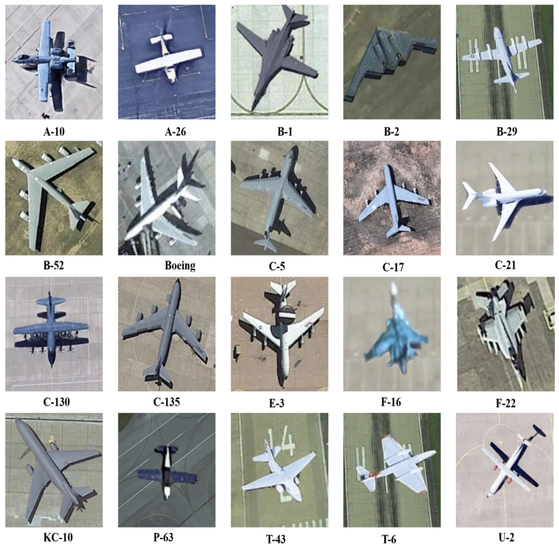
The multitype aircraft remote sensing images (MTARSI) dataset represents the first public, fine-grained aircraft type classification dataset for remote sensing images. Seven specialists in the field of remote sensing image interpretation painstakingly labeled all of the example images. Thus, this dataset possesses high authority. Overall, MTARSI has collected 9385 remote sensing images from Google Earth satellites. Boeing C-5, P-63, T-43, B-1, KC-10, C-130, B-2, B-52, B-29, C-135, C-17,E-3, F-16, C-21, U-2, A-10, A-26, T-6, and F-22 aircraft are included in the 20 aircraft images in the dataset. The number of sample images for different aircraft types is different (see
Table 1) and ranges from 230 to 846. In other words, the number of different types of aircraft is imbalanced, which increases the difficulty in aircraft type recognition. Furthermore, the MTARSI includes pictures with varying spatial resolutions as well as complex changes in posture, geographic position, lighting, and time period. This aspect enriches the intra-class variation, rendering aircraft type recognition more challenging. Furthermore, all the aircraft types are similar in appearance and difficult to distinguish, and thus certain inter-class similarities exist in the dataset for each aircraft type. Several examples of aircraft images in the MTARSI dataset are shown in
Figure 3.
4.2. Evaluation Metrics
In the experiments, we adopted the accuracy and confusion matrix to quantitatively evaluate the aircraft recognition performance. The confusion matrix is a visualization tool that reflects the classification performance of the model, especially for supervised learning. The matrix was determined by comparing the position and classification of each measured pixel with the corresponding status and category in the classified image.
4.3. Implementation Details
Parameter-settings: To effectively extract the features, we followed the AlexNet parameter settings to set the parameters of the BD-ELMNet, as shown in
Table 2, which summarizes the parameters such as the convolution kernel size, number of feature maps, and pooling size. We selected hyper-parameters through cross-validation, such as the number of hidden nodes k in the autoencoder (MRELM-AE), the normalization parameter C and
. As shown in
Table 3, the number of hidden neurons ranged from 100 to 5000, and the interval of all AEs was 100. We selected the hyperparameter C in the range of the exponential gap [1.0 × 10
, 1.0 × 10
] based on the validation set test results.In addition, we set the activation function of the ELM as a non-linear sigmoid function.
Programming-environment-settings: As the experimental platform for all experiments, we used a PC with an Intel i7-6700 CPU, 2.60 GHz, 8 GB of RAM, and GeForce GTX 1080ti GPUs. The algorithms were implemented and executed in MATLAB 2020b.
4.4. Hyper-Parameter Study
The key hyperparameters that affect the performance of BD-ELMNet are mainly the balance parameters , and the number of hidden neurons . We performed multiple crossover experiments to determine the hyperparameter values.
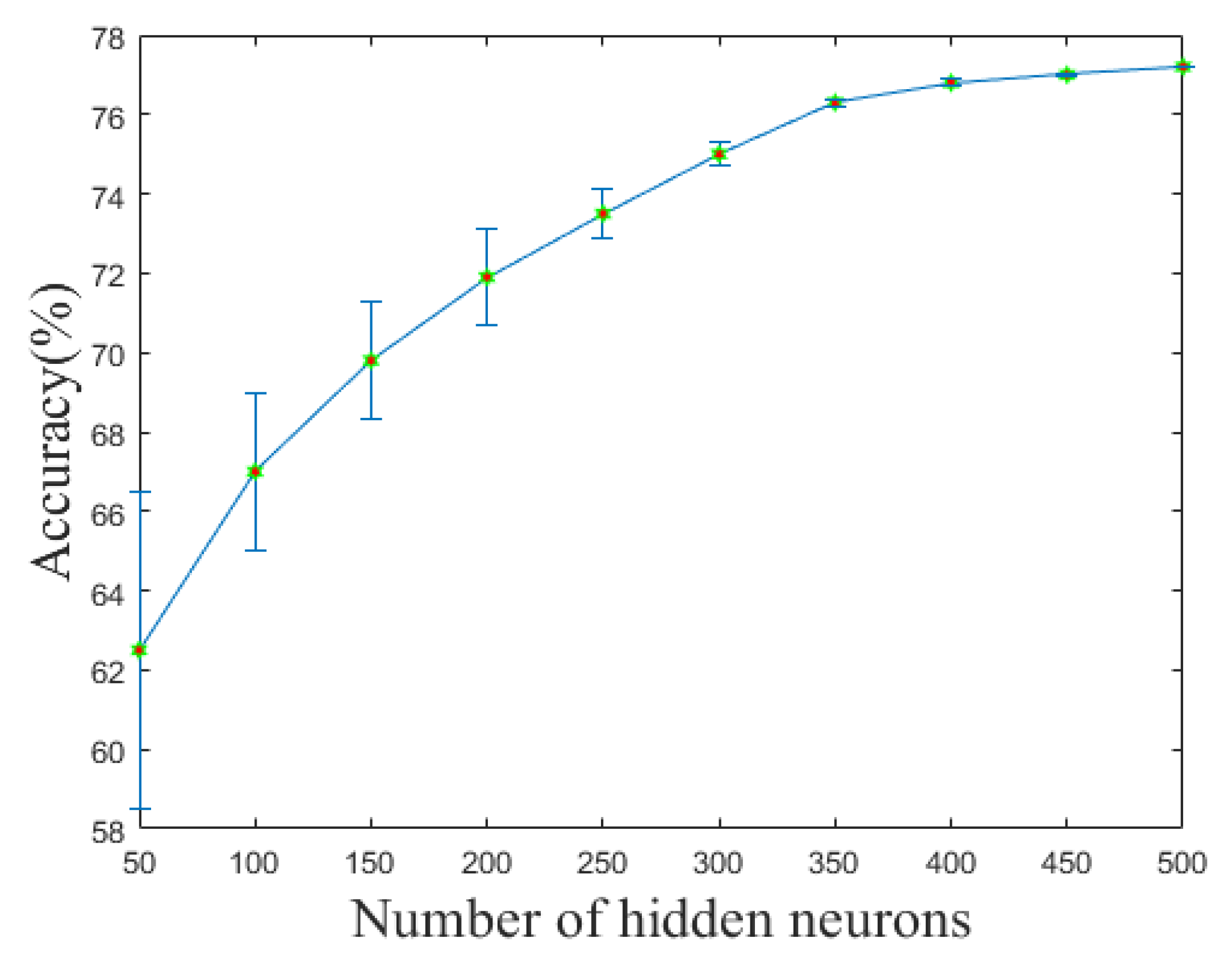
Selection of the number of hidden neurons. We studied the effect of the number of hidden neurons k on the accuracy of aircraft recognition in this experiment. As shown in
Figure 4, as the number of buried neurons increased, the algorithm obviously achieved better accuracy and a lower standard deviation. Even with a larger number of buried neurons than 300, the average accuracy remained constant, ranging from 72.15% to 77.1%. When there were more than 450 hidden neurons, the standard deviation was less than 0.05. As a result, we set the number of hidden neurons to 450 in the next trials.
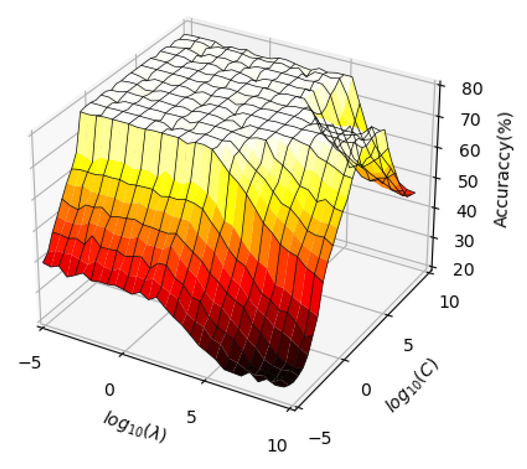
Selection of the balance parameters. The purpose of this experiment is to determine the effect of limited parameters on the accuracy of aircraft recognition.
Figure 5 shows the recognition accuracy for different combinations of parameters and
. Clearly, the accuracy of aircraft recognition tends to be stable when
and
.
4.5. Ablation Studies
We provide various comparisons in
Table 4 to assess the contribution of each module, where the MRELM-AE, bilinear pooling, and W-ELM correspond to the BD-ELMNet. First, we evaluated the contribution of several elements to our baseline recognizer as a reference. As shown in
Table 4, all the techniques contributed to an increase in accuracy, and the final baseline attained an accuracy of 0.781.
(1) Convolution-pool layer. We expanded the single-layer ELM-LRF to a multi-layer neural network structure by introducing multiple convolution and pooling operations. A deep neural network structure can not only extract the abstract information of the image but also can ensure the displacement invariance of the data feature attributes. An increment of 4.9% was achieved. This finding proves that the multi-layer convolution-pooling operation can enhance the feature extraction ability of the ELM-LRF.
(2) MRELM-AE. The MRELM-AE achieved a performance enhancement of 3.8% compared to that of the baseline. This finding shows that the discriminative features learned by the MRELM-AE can effectively increase the accuracy of target recognition.
(3) Compact bilinear pooling. In comparison with the baseline, compact bilinear pooling achieved certain enhancements, which may be attributed to its ability to extract the pairwise correlations between feature. The relative increase was approximately 8.9% in aircraft type recognition tasks.
(4) W-ELM. The performance gain (approximately 6.4%) associated with the W-ELM was relatively large due to the use of the weighted classification cost function, which can mitigate the impact of the category imbalance problems in the considered tasks.
4.6. Comparison with State-of-the-Art Methods
On the MTARSI dataset, we compared the proposed BD-ELMNet with various similar techniques to evaluate the efficacy of the proposed methods; see
Table 5. The following related methods were considered: (1) Handcrafted-feature-based approaches: BOVW [
78], LBP–SVM [
79]. (2) Deep-learning-based approaches: PCANet [
24], SqueezeNet [
47], AlexNet [
12], MobileNet [
61]. (3) ELM-based approaches: ELM-LRF [
27], ELM-CNN [
75].
The handcrafted-feature-based approaches [
78,
79] are state-of-the-art methods in the field of image recognition; thus, we compared these methods with the proposed method. We utilized a fixed grid size (
pixels) with an interval step of 8 pixels to extract all the descriptors in the picture for local patch descriptors such as the SIFT, and we used the average pooling pixels in each dimension of the descriptors to obtain the final image characteristics. For the BOVW, we set the dictionary size at 4096.
In addition, to perform comparative analysis, we applied deep-learning-based approaches and ELM-based approaches. Among these methods, SqueezeNet and AlexNet require the BP algorithm for iterative optimization, while the PCANet, ELM-LRF, and ELM-CNN do not require trivial BP fine-tuning. Note that both AlexNet and LeNet are trained from scratch, and ImageNet-based pre-training models are not used. Furthermore, the PCANet and ELM-LRF methods have two hidden layers. The MTARSI dataset is divided into training and test sets in a ratio of 7:3, and the size of the images is fixed as pixels. To ensure a fair comparison, the abovementioned methods were compared according to the training set and test set.
Table 5 indicates that the BD-ELMNet, MobileNet, SqueezeNet, AlexNet, and ELM-CNN exhibit the highest performance, which demonstrates that deep learning based on multi-layer network feature learning can help to learn strong distinguishing features from shallow to deep learning. Since shallow learning methods such as the PCANet and ELM-LRF have only two hidden layers, their feature expression ability is weak and cannot overcome the problem of indistinguishable aircraft with similar shapes.
The performance of the methods based on manual features is lower than that of AlexNet and the proposed method. In particular, the manual feature methods cannot effectively overcome the interference of factors such as illumination and rotation, although a method based on deep learning can independently learn robust features. The BD-ELMNet performs somewhat better than deep learning methods such as AlexNet, demonstrating the method’s efficacy. This finding shows that the bilinear pooling and manifold regularization can be used to effectively enhance feature discrimination.
Table 6 presents the experimental results of the different classification algorithms in terms of the computational complexity.
The suggested method’s training duration was compared to that of the SqueezeNet, MobileNet, and AlexNet techniques in order to assess its computational efficiency and show its recognition accuracy. As indicated in
Table 6, the training speed of the shallow learning network (not requiring BP adjustment) was considerably higher than that of the deep learning network. The training time of the BD-ELMNet was higher than that of the ELM-LRF and ELM-CNN because its network involved the additional MRELM-AE and bilinear pooling module. Compared with SqueezeNet, MobileNet, and AlexNet, the training time of BD-ELMNet was reduced by three times, which proves that the layer-wise training procedure can shorten the training time compared with that of the BP optimization method. Since they have a non-convex function, deep learning methods such as SqueezeNet require BP optimization to perform multiple iterations of training to find the local optimal solutions.
To prove the effectiveness of the proposed BD-ELMNet algorithm on the small-scale MSTARSI dataset, we conducted performance tests by using three classical deep learning algorithms, namely AlexNet, SqueezeNet, and MobileNet, with different training methods. We trained these deep learning networks from scratch and trained them with the ImageNet pre-training models. In these two training methods, we added a data augmentation method based on image transformation. The training results are summarized in
Table 7.
The following observations can be made from
Table 7: (1) the effect of the training method fine-tuned using the pre-training model is superior to that of the method trained from scratch; (2) although the proposed method adopts the method of training from scratch, its effect is superior to that of the deep learning algorithm trained using the pre-trained model. The first observation demonstrates that the use of pre-trained models to fine-tune training can alleviate the problem of model overfitting caused by small samples. Such a pre-trained model that is easy to generalize is obtained after training with a large number of sample sets similar to ImageNet. Compared to training using the ImageNet pre-training model, even if the data-enhanced de novo training method is adopted, the effect is far poorer than that of the training method in which fine-tuning is performed using the pre-training model. The above observation can be attributed to three main reasons: (1) the feature learning spaces of deep learning models such as AlexNet are high-dimensional spaces. As the dimensionality increases, the number of samples required increases exponentially. Small samples can easily lead to overfitting when overly complex training models are used. (2) Deep learning models such as AlexNet are nonconvex optimization models with high nonlinearity. The nonconvex optimization method often uses gradient descent optimization, which leads to limited changes in the parameters of each node when the sample size is limited, causing deep learning to easily fall into a local optimum. (3) Deep learning uses only the data calibration drive mechanism, only relevant learning abilities, and no causal reasoning ability of knowledge rules. (4) Even if the data augmentation method is used to enhance the sample size, the enhanced sample size cannot reach the level of ImageNet in terms of magnitude or diversity, and for this reason, a deep learning algorithm with the above shortcomings cannot perform well in terms of feature generalization. The second observation indicates that the proposed method is superior to deep learning models when applied to small sample datasets. The reasons for this are as follows: (1) The proposed method draws on the ELM optimization strategy, and the ELM model seeks the global optimal solution. The hidden layer ELM parameter must learn only its output layer weight parameters. Unlike classical deep learning, which uses cumbersome iterative adjustment strategies for all network parameters, the hidden layer node parameters of the ELM network need not be adjusted, meaning that the output layer parameter solution is transformed into a simple linear optimization problem. This linear convex optimization method reduces the training time and reduces the dependence on sample size. (2) We adopt unsupervised layer-by-layer training methods, such as autoencoders, for the multi-layer network structure. The layer-by-layer training strategy helps us to determine the “good” initial values of the parameters to be optimized, which facilitates rapid convergence in the subsequent global iteration process. The sample size required for the parameter adjustment of the layer-by-layer pre-training strategy is considerably smaller than that for the BP optimization method. (3) In terms of feature expression, the proposed method not only draws on the mechanism of the local receptive field of CNNs but also on popular regularization and bilinear pooling ideas to enhance its feature expression ability. Compared to deep learning that uses only convolutional feature extraction, the feature expression ability of the proposed method is slightly superior.
4.7. Analysis of the Image Features in MTARSI
Considering the results of the experiments involving different classification algorithms, we investigated the type of aircraft in the MTARSI dataset that is most likely to be misidentified. First, we considered the recognition rate for each airplane using various categorization techniques, and then we determined the kinds of aircraft that were most often confused.
Figure 6 provides the confusion matrices for the LBP–SVM, BovW, ELM-LRF, ELM-CNN, PCANet, SqueezeNet, AlexNet, and BD-ELMNet on the MTARSI dataset.
The methods based on manual features and shallow learning exhibit a certain recognition performance; however, many misclassifications of similar aircraft types (such as C-5 and Boeing or B-52) occur. This phenomenon occurs because the method based on manual features lacks discriminative representation, thereby rendering it difficult to distinguish airplanes with similar shapes when using manual feature methods.
Moreover, the shallow learning method has limited learning feature patterns, and it is challenging to cover multiple aircraft types. Therefore, the associated recognition ability is inferior to that of the deep learning network. In comparison to the two techniques described above, the deep learning method based on multi-layer network feature learning can learn numerous templates related to aircraft structural characteristics using many convolution kernels, improving the deep learning method’s feature expression capabilities. However, AlexNet and ELM-CNN methods still struggle to distinguish similar aircraft. These deep-neural-network-based methods do not consider the essential characteristics of the data points, such as the local and global geometries. According to
Figure 6h, the proposed method demonstrates an excellent performance except on certain extremely similar aircraft. The main reason is that our method preserves the local geometry and exploits the local discrimination information from the input data. The study experimentally demonstrates that the proposed method can learn data representations with a maximized within-class compactness and between-class separability.


