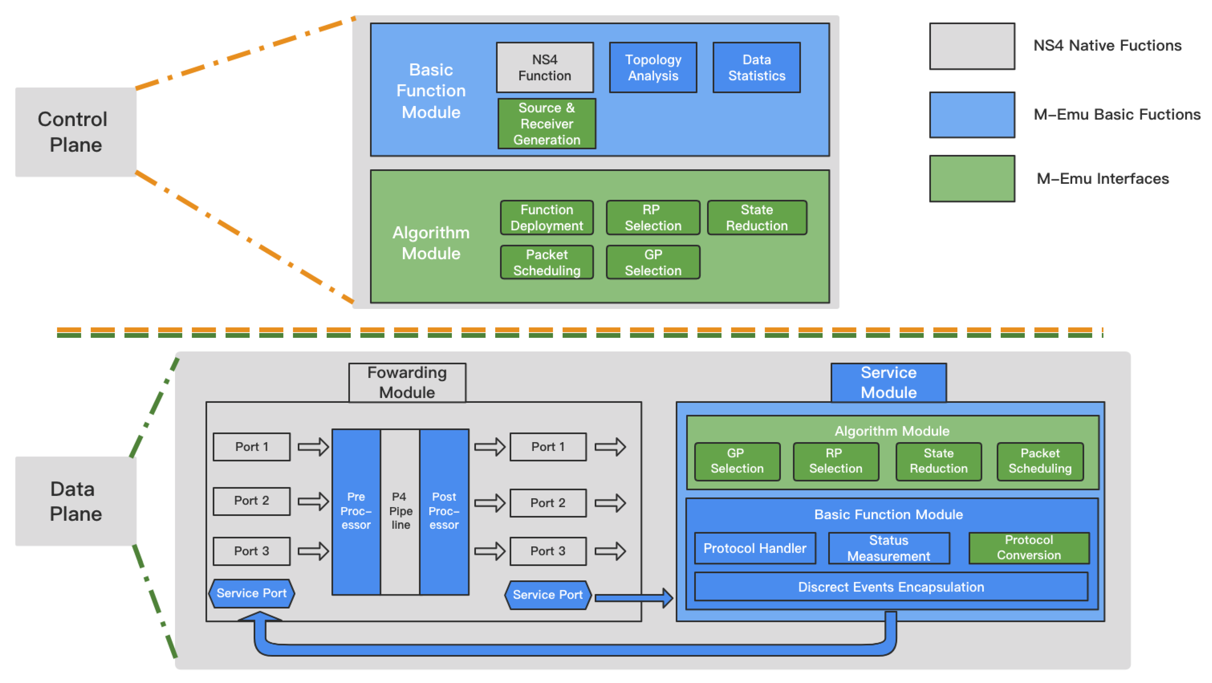
In this part, we explore the effectiveness and efficiency of M-Emu. First, we take PIM-SM emulation as an example to introduce how M-Emu can effectively support the emulation of various multicast technologies. Secondly, we compare the differences between M-Emu and the original NS4 in terms of CPU usage and memory usage, etc., when deploying the PIM-SM emulation.
4.1. Case Study
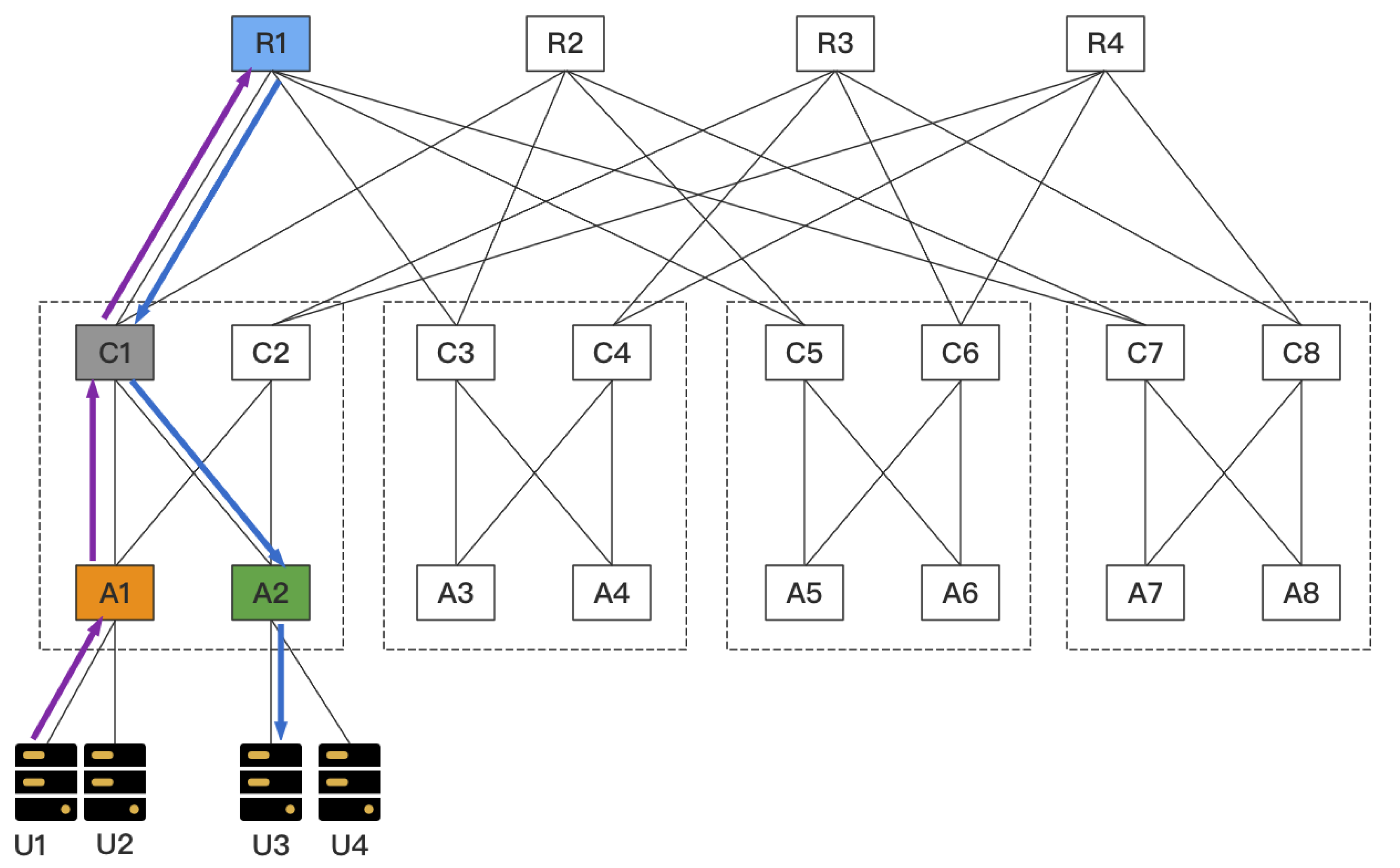
We take the emulation of PIM-SM as an example to explain in detail how the various parts of M-Emu cooperate to complete the multicast emulation. We emulate PIM-SM in a fat tree topology, which is shown in
Figure 4.
PIM-SM is the most popular IP multicast at present. The multicast tree of PIM-SM is a Shared Tree. Each source DR selects a node from the cRPs set as the RP. Each receiver-side DR then selects this RP as GP. First, we need to deploy the DRs. M-Emu provides the DR deployment interface, which is
void SetDR(
std::map < std::string, Ptr > nodeMap,
const NodeContainer nodes,
NodeContainer* senderDR,
NodeContainer* receiverDR)
Among the parameters of this interface, std::map < std::string, Ptr > nodeMap maintains the map** between the node ID in the topology file and the node ID in the emulated network. A topology file is a file provided by users that describes the topology. The emulators or simulators can build a topology based on this file. The nodeMap is adopted because these two IDs are often inconsistent. const NodeContainer nodes contains all nodes in the topology. NodeContainer* senderDR and NodeContainer* receiverDR, respectively, store the pointers of the source-side DRs and receiver-side DRs. In this example, we add A1 to senderDR and A2 to receiverDR. The simplest way to do this is to find the IDs of A1 and A2 from the topology file, then use the nodeMap to find the node pointers of A1 and A2, and finally add them to the corresponding nodeContainer.
Second, we deploy the cRPs. M-Emu provides the RP deployment interface on the control plane, which is
void SetRP(
std::Map < std::string, Ptr > nodeMap,
const NodeContainer Nodes,
NodeContainer * cRPs)
NodeContainer *RP contains pointers to all cRPs. In this example, we add R1, R2, R3 and R4 to this nodeContainer.
When A1 receives data from U1 or U2, A1 runs the RP-selection method to select a node from the cRP set as the RP. M-Emu provides the RP-selection method interface on both the control plane and data plane, which is
uint32_t GetRootNode(
const NodeContainer cRPs,
uint8_t * buffer, void* info)
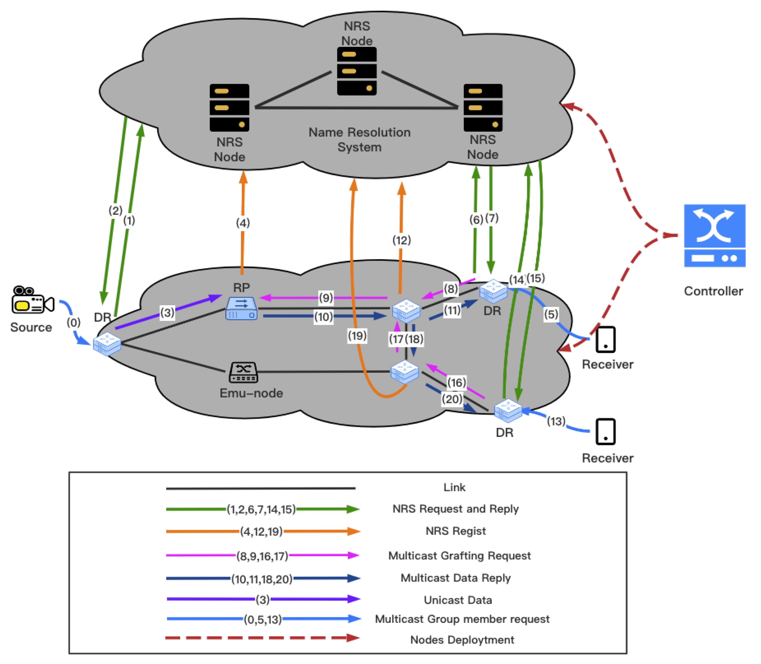
The return value of this interface is the ID of the RP we selected. uint8_t* buffer holds the multicast data. void* info contains external information on which the algorithm depends. The control plane can add some global information to info, while the data plane can add only local information to info. We approximate that PIM-SM selects the RP using the hash of the multicast ID, which is provided in uint8_t* buffer. In this example, we assume that A1 selects R1 as RP for the current multicast group.
After receiving the multicast data, R1 will register the map** between its NA and multicast ID with NRS, as described in the previous section. At some point, A2 will receive a data request from U3. A2 runs the GP-selection method to select a node from the multicast tree as GP. M-Emu provides a GP-selection algorithm interface on both the control plane and data plane, which is
The return value of this interface is the ID of GP. The difference between the control plane and the data plane of the interface is still reflected in the content of the info. In this example, the DR on the receiver side selects the root node as GP each time. To find the address of the root node, the DR queries the address list of nodes in the multicast tree from the NRS based on the multicast ID in uint8_t * buffer. The first node in the list is the root node, because in every multicast tree, the first node to register with the NRS must be the root node.
When R1 receives a joining request from A2, it sends multicast data back to A2. When the multicast data passes through C1, C1 determines whether to create the MFT entry based on the State Reduction method. M-Emu provides the interface on both the control plane and data plane, which is
If the return value of this interface is 0, the node should not register MFT entries. In this example, each node should register the MFT entry; therefore, when a node runs this interface, the return value is 1. The whole process of the emulation is shown in
Figure 5.
After the above process, a multicast tree can be established in PIM-SM mode. According to
Section 3.3, the
Statistical tools provided by M-Emu records data packet information in a certain format. Next, we give an example of how M-Emu records packet information.
After A1 selects R1 as its RP, it sends data to R1 by unicast. When R1 receives multicast data from A1, it records the data as
Figure 6. The meaning of the data in
Packet Type can be found in
Section 3.2. When C1 forwards the multicast data sent from R1 to A2, the multicast data is recorded as shown in
Figure 7. When A2 receives multicast data from R1, it records the data as shown in
Figure 8. It can be seen that
Statistical tools can accurately and comprehensively record the forwarding status of multicast packets on the network.
According to the data packets recorded by all nodes, we can find the following key information:
MFT load: R1, C1, A1 and A2 all need to maintain the multicast forwarding state for this multicast group, and thus their MFT load is +1.
Link Load: Links R1-C1, C1-A1 and C1-A2 all need to forward the multicast stream, and their load is 100 Kb/s.
Multicast tree cost: The multicast tree forwards 100 bits of data through three links. Therefore, the Multicast tree cost is 300 bits.
End-to-end delay: According to the time stamp of each data packet, the time of sending data from A1 to A2 is 5 ms.
In many cases, users want to emulate SBT rather than ST. At this point, the user simply adds each DR to the cRPs set and forces the DR to select itself as the root node. In addition, users can also adjust the RP-selection method and GP-selection method to build a more complex multicast tree.
4.2. Emulation Performance
In this part, we test the performance of M-Emu and original NS4 in various aspects when deploying the experiments in
Section 4.1. We require the data plane to execute multicast algorithms independently without interaction with the control plane. The reason for such a setting is that many researches require the data plane to have the ability to independently formulate and execute various algorithms [
12,
13,
15].
For NS4, to enable the data plane to handle multicast protocols and algorithms independently, a natural thought would be to add a host, which we can call a service node, directly connected to each switch. The service nodes of NS4 operate as the service module of M-Emu, while the switch nodes of NS4 operate as the forwarding module of M-Emu. This approach is a degradation of M-Emu because it requires the deployment of additional nodes, resulting in increased system resource usage. Our experiments are conducted on a Dell R740xd PowerEdge server with two Xeon(R) Gold 5218R CPUs and 300 GB RAM.
The evaluation metrics include:
Memory Consumption. This metric indicates the memory size required by the emulation platform to process a certain number of multicast flows.
CPU utilization. This metric indicates the CPU utilization by the emulation platform to process a certain number of multicast flows.
Traffic of Management Message. This metric indicates the traffic of various management messages when the same number of multicast flows (1000) are completed.
Packet Process time of Emu-Node. This metric indicates the time required for the emulation platform to interact with the real network.
Execution Time. This metric indicates the time required by the emulation platform to process a certain number of multicast flows.
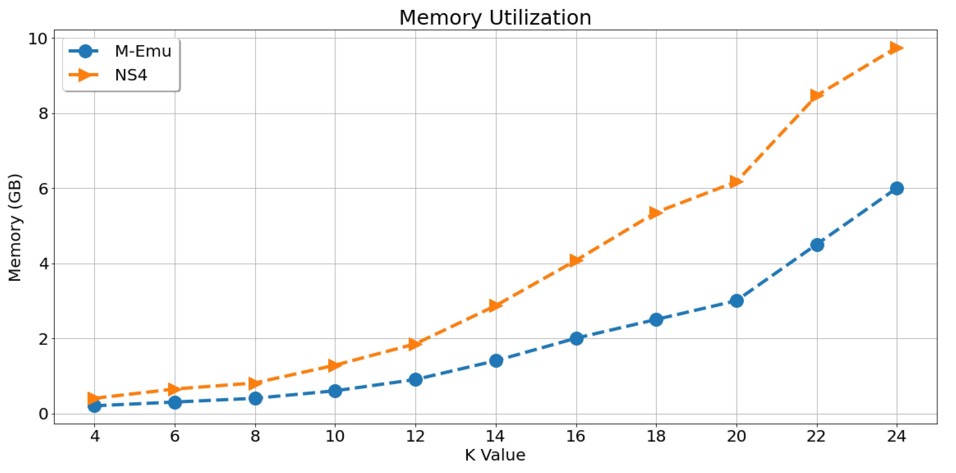
4.2.1. Memory Consumption
We compare the memory consumption of each architecture in fat tree topologies when processing 1000 multicast flows. The results are shown in
Figure 9. It can be seen that, with the increase of K, which indicates the size of fat trees, the memory consumption of both architectures increases gradually. This is because both M-Emu and NS4 need to populate routing entries in every switch. The larger the topology is, the more memory the flow tables occupy. Furthermore, the memory consumption of M-Emu is about 60% of that of NS4, Thus, compared to NS4, M-Emu can save more memory. This is because NS4 requires service nodes, which makes the topology of NS4 larger and the memory consumption of the flow tables higher.
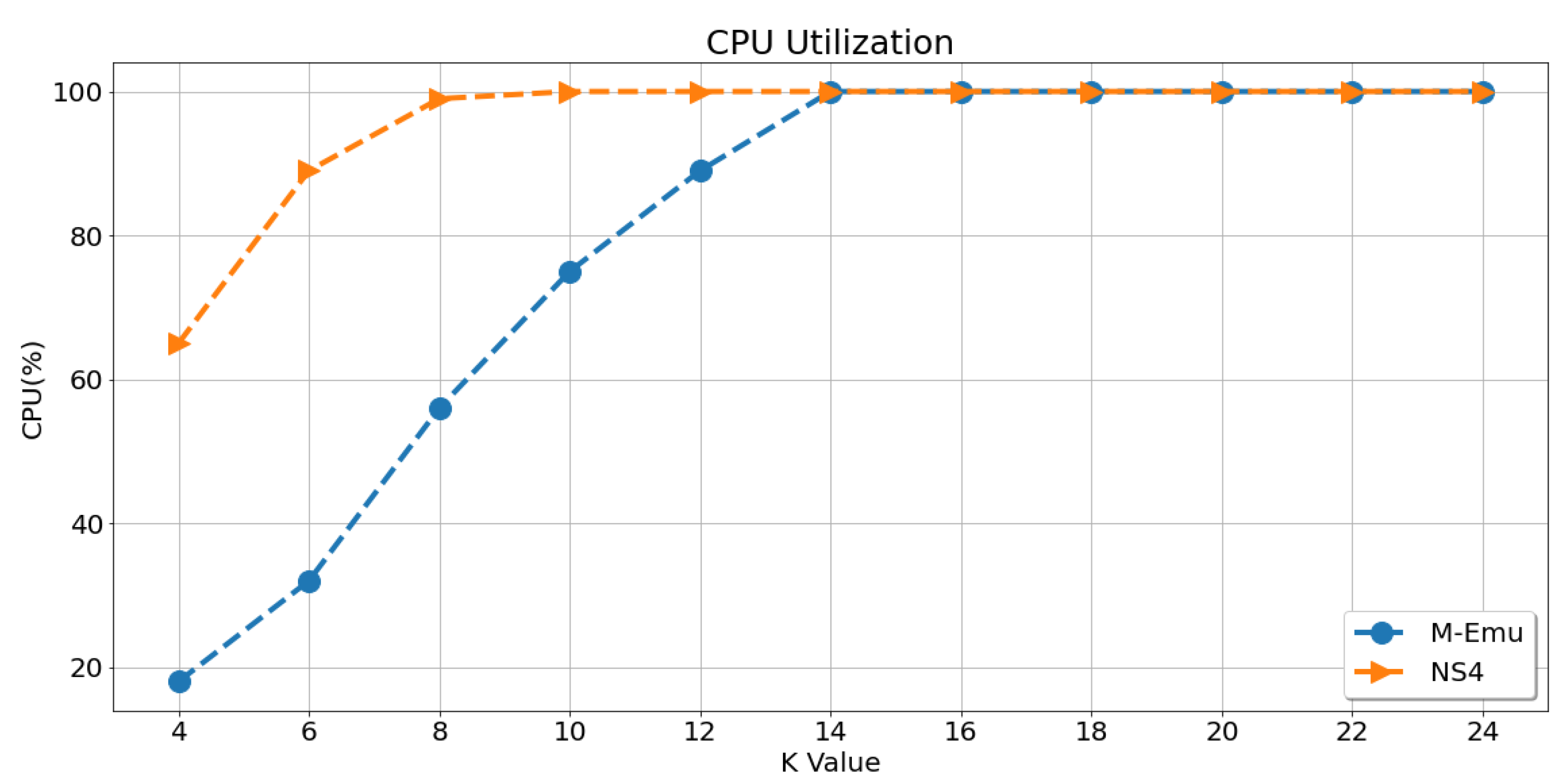
4.2.2. CPU Utilization
In this part, we compare the CPU consumption of each architecture in fat tree topologies when processing 1000 multicast flows. The results are shown in
Figure 10. It can be seen that, with the increase of K, the CPU utilization of M-Emu rises slower than that of NS4. When K = 4, the CPU utilization of M-Emu was about 30% of that of NS4. This is because NS4 needs to forward packets from switches to service nodes, and it also needs to parse or encapsulate packets from the link layer to the application layer on the service nodes.
Both actions can be omitted in M-Emu. The service module and forwarding module of M-Emu are connected by queues, avoiding the addition of NetDevices and Channels in the network, which are two basic units of ns-3 or NS4. Furthermore, the service module in M-Emu can directly check specific fields of data packets according to offsets, which greatly improves the analysis efficiency. Therefore, the CPU usage of M-Emu is lower than that of NS4 when processing multicast protocols.
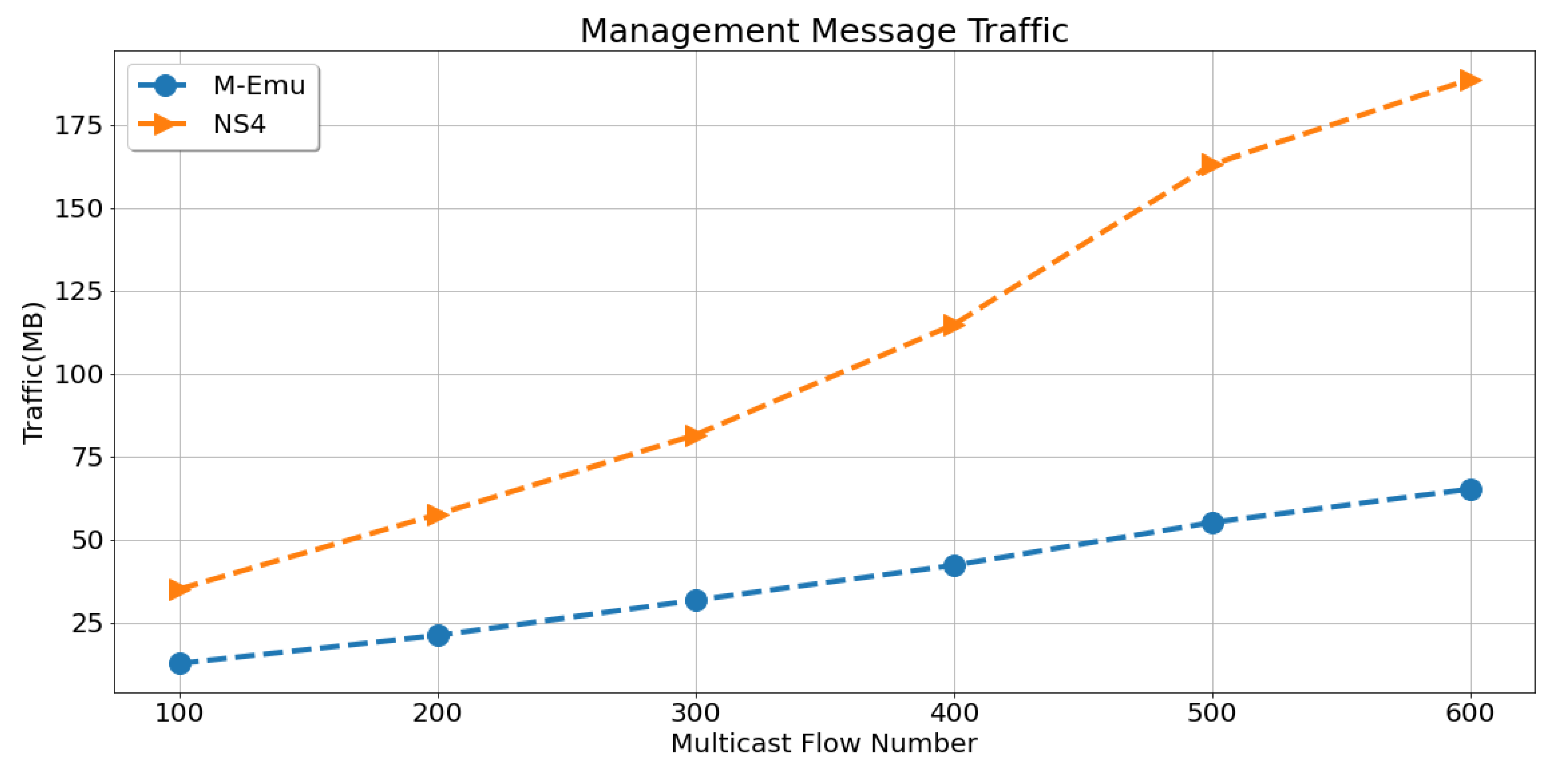
4.2.3. Traffic of Management message
In a fat tree topology with K = 6, we compare the management traffic required by each architecture when processing the same number of multicast flows. The management traffic refers to the traffic of multicast tree establishment and maintenance message. As can be seen from
Figure 11, as the number of multicast flows increases, the management traffic of each architecture increases. The traffic of management messages of M-Emu is about 1/3 of that of NS4. This is because, for NS4, the traffic between service nodes and switch nodes accounts for about 2/3 of the total control management traffic, and this part of the traffic can be omitted in M-Emu.
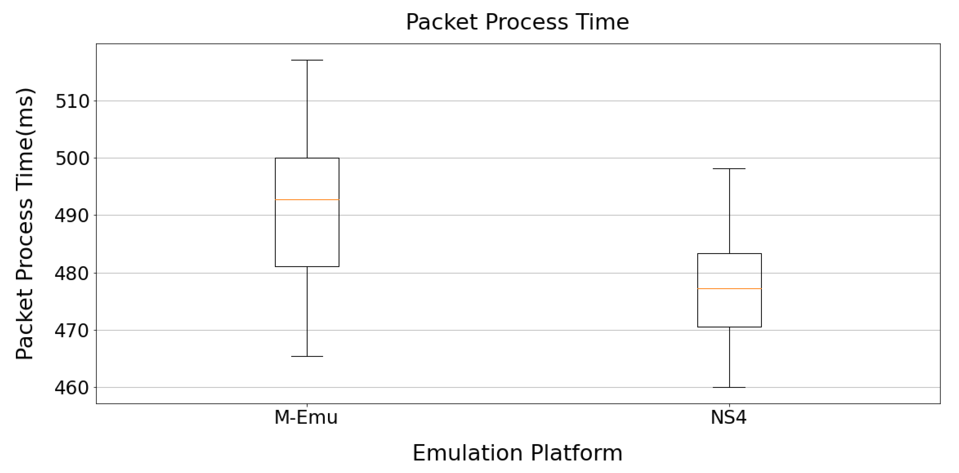
4.2.4. Packet Process Time of Emu-Node
Since the protocol conversion module of M-Emu needs to modify the header of each packet, the packet processing delay will increase slightly on Emu-node compared with NS4. We ran 1000 packet interactions with the real environment and compared the packet processing time of M-Emu with that of NS4. The results are shown in
Figure 12. It can be seen that the modification of the packet header does increase the packet processing time slightly, by about 3% compared with NS4.
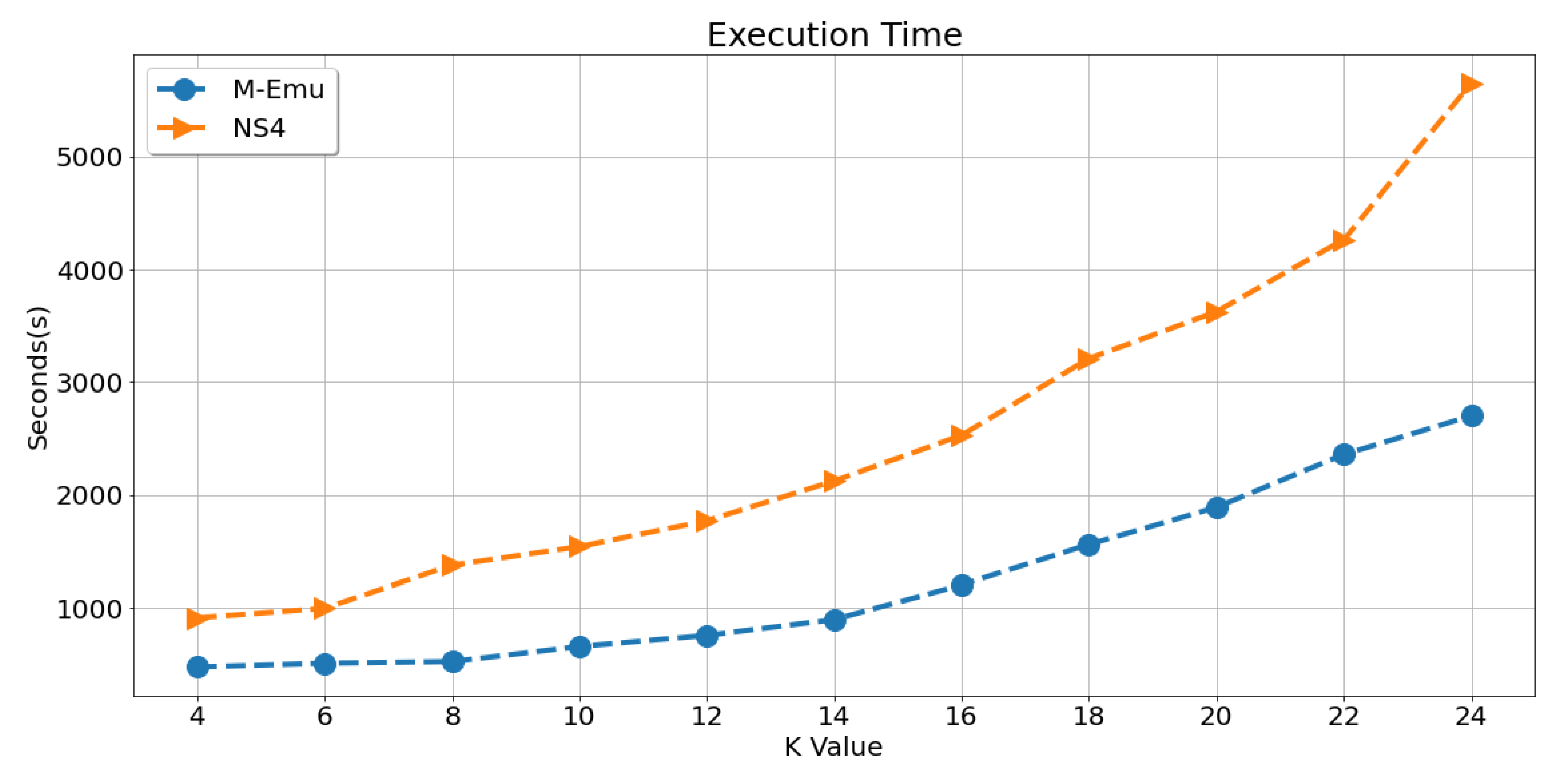
4.2.5. Execution Time
In this part, we compare the execution time required by each architecture when processing the same number of multicast flows (1000 multicast flows). The execution time is related to many factors, such as the memory consumption, CPU utilization and so on; thus, it is a comprehensive factor to measure each architecture’s performance. The results are shown in
Figure 13. It can be seen that, with the increase of K, the execution time of these architectures increases gradually. The execution time of M-Emu is about 1/2 of that of NS4.
This is mainly because: (1) In NS4, the communication delay between service nodes and switches increases the complete time of a multicast flow, thus increase the total execution time. (2) The topology size of NS4 is almost twice as large as that of M-Emu. The larger the topology is, the more resources the experiment consumes and the slower the experiment runs. (3) The packet processing logic on the service node is more complex than that of M-Emu’s service module. Thus, the Execution Time of NS4 is much larger than that of M-Emu.
4.2.6. Code Complexity
In this section, we make a comparison between M-Emu and NS4 in terms of the code complexity (number of lines of code). Since M-Emu is an improvement on NS4, M-Emu has much more code on both the control plane and data plane than does NS4. The results are shown in
Table 3.
We only counted the amount of code in the source file. It can be seen that the code quantity of M-Emu is larger than that of NS4 in all modules. In the forwarding module, because M-Emu only adds ports to the service module, there is not much more code than for NS4. As NS4 has no service module, the code quantity of its service module is 0. However, M-Emu has the multicast simulation function deployed in the service module, and thus the code quantity is much larger than NS4.


