1. Introduction
Published works on UAV systems confirm that these systems currently have a wide range of applications. UAV systems can be used for terrain monitoring to protect state borders, for terrain scanning in agriculture, in the military for reconnaissance and attack missions, for monitoring important objects, etc. The advantage of using UAVs is their low price, relative autonomy in the activities performed, and the possibility of multiple use [
1,
2]. The increased demand for UAVs results from the increasingly complex environment of the performed reconnaissance and monitoring missions. A significant problem is represented by monitoring tasks that require high performance in terms of autonomous orientation and communication in the space of the ongoing mission. However, a single UAV can hardly meet its actual task requirements because its sensor’s field of view can be easily blocked, limiting its ability to perform tasks [
3]. The cooperation of several drones should eliminate these situations and ensure more accessible and stable monitoring of the area. Currently, multi-UAV collaborative planning using the artificial potential field method, bionic algorithm, or control algorithm is analyzed in [
4,
5]. In the case of using the artificial potential field method for collaborative planning, it is possible to slip into local optimality. Then, it is challenging to create a mathematical model of UAV trajectories. In the case of ant colony and particle swarm bionic algorithms, it is difficult to satisfy the real-time demand due to their limited processing efficiency [
6,
7]. Animesh Sahu [
8] and others created a study on object movement tracking using UAVs in two dimensions based on a predictive control algorithm model. The model is based on the Gaussian Process (GP), which combines the hyperparameters used in the predictive control phase and significantly impacts mission efficiency. A comprehensive analysis of the above research found that most current research on multi-UAV trajectory planning through cooperative formation has been conducted in two-dimensional space. This results in limitations, such as the computational complexity of the large-scale model and the long time for real-time computation. At the same time, current research needs help in creating a complete non-linear 3D movement model of the UAV, which results in difficulty in meeting the actual requirements related to the mission objective [
9]. As for the traditional multi-UAV sensors, their working areas need to be improved. Low data formation and retention capabilities prevent them from becoming a hot candidate for use in this field [
10]. Multi-UAV formations, control, communication, and computer processing of time data must be complemented by distributed control strategies, which present higher requirements for the multi-UAV formation. A typical multi-UAV system is a multi-agent system [
11]. The user can measure the relative distance from the neighboring user and guide the controlled shift to the next UAV. In this way, the desired formation can be achieved. There needs to be more control of their mutual positions. Because of this, they do not have the same sense of direction. There are also many studies on the cooperative creation of UAV control [
12,
13], which provide path planning, optimal perceptual geometry, distributed control law design, and information architectures. Multi-UAV cooperative trajectory planning (MUCTP) is planning multiple safe and collision-free flight trajectories based on the spatial location of UAVs, mission points, and obstacles in a complex planning environment [
14,
15]. The planned trajectory of a single UAV can hardly handle complex missions due to its limited maneuverability and payload. MUCTP has the advantage of being more flexible and efficient in carrying out missions than standalone UAV assets. For this reason, when performing complex missions, this solution is gradually replacing using separate UAVs. However, MUCTP also increases the difficulty of planning the trajectory of UAVs. In cooperative planning, the self-constraints of heterogeneous UAVs and the mutual constraints between multiple UAVs may lead to conflicting relationships and disturbances between each UAV and the mission point, ultimately leading to mission failure [
16,
17].
In recent years, to improve the efficiency of MUCTP scheduling, researchers have proposed many algorithms that have shown good performance in solving MUCTP problems, and these algorithms are mainly divided into three categories:
Cooperative trajectory planning based on intelligent optimization algorithms
Cooperative trajectory planning based on reinforcement learning
Cooperative trajectory planning based on the spline interpolation algorithm
Based on the algorithms presented in [
17], it is possible to design the architecture of an anti-collision system for UAVs that can determine the position of the UAV relative to other users in the air communication network. The condition for the functioning of these algorithms is that all flying objects communicate with each other. The results of the research work on the anti-collision system with the radar obstacle detector are discussed in [
18]. The main tasks set for this system are detection of static and moving obstacles, estimation of the distance between the flying object and the obstacle, and their relative speed. Most cooperative obstacle avoidance strategies use Wmethod. The APF method [
19,
20] is widely used in the design of anti-collision systems for cooperative UAV formations. The algorithm relies on the creation of gravitational and repulsive fields to calculate the resultant force that determines the path planning at each moment. However, if the chosen design of the field function is incorrect, the APF algorithm may fall into the local optimal solution. Another disadvantage of the implementation of this method is the fact that it does not take into account the limitations of the dynamic movement of the UAV, which makes it difficult to track the planned path in real time. Based on the research of ** the models, we have abstained from the forces’ influence on the UAV during the flight. We assume that this approximation is relevant for verifying the accuracy of determining the position of the selected member of the group.
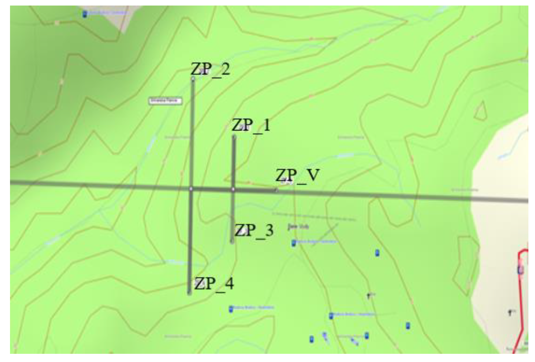
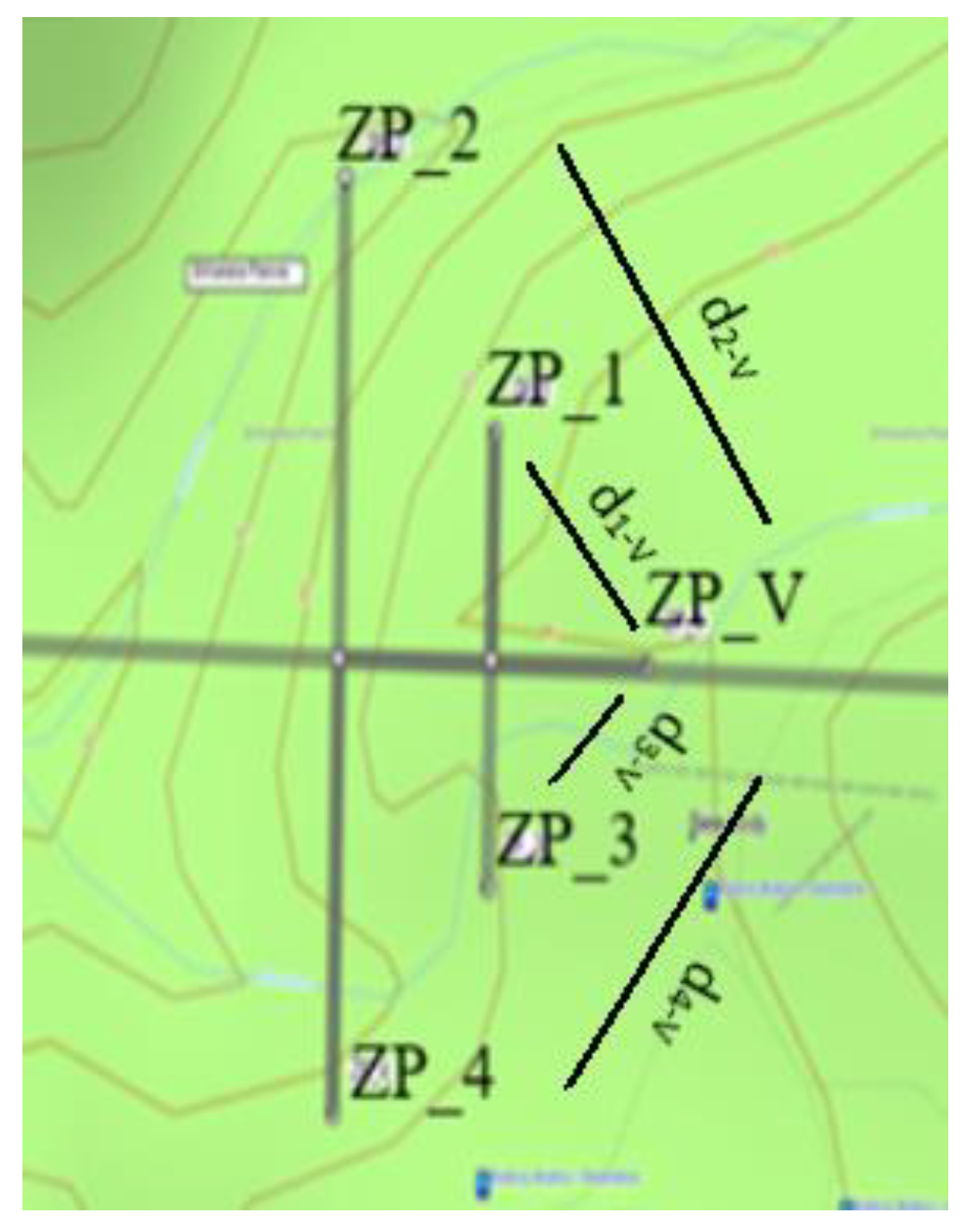
In
Figure 1, ZP_V is the initial position of the leader of the group of UAVs, and ZP_i, i = 1, 4 are the initial positions of the members of the group of UAVs, 1 to 4. Other group members, at designated distances for the flight duration, follow the group leader. Based on data from other UAVs, other group members determine its position. The coordinates of the initial position of the members of the UAV group are shown in
Table 1. When creating a model of the movement of five flying UAVs, they chose the formation they would fly in. At the head of the formation is the leader of the group, and to its left and right sides are two UAVs. In develo** the model, a condition was observed that the maximum distance between the group’s leader and any group member should not exceed 1000.0 m. We assumed that the group would form in the surrounding area of the Sliač airbase and fly eastward at an altitude of 1850.0 m. The initial position of the group is shown in
Figure 1. The distance between group members is at least 300.0 m.
We assumed that these coordinates are considered to be the reference and represent the start point of the flight trajectory, , where . When modeling the movement of a group of UAVs, we set the condition that this group’s flight trajectory will contain one rectilinear section and three curvilinear sections in the shape of a circle.
We can set the initial parameters of the flight modeling of five UAVs by the task solved by the UAV group. The parameters of the models that can be entered are the initial positions of the UAV, the time of rectilinear flight, and flight, in turn, including its radius. Another requirement for the motion models was to determine and visualize the positions of the UAV in the ECEF rectangular coordinate system. The positions of the UAV must be determined according to the selected period by x, y, and z coordinates, in meters.
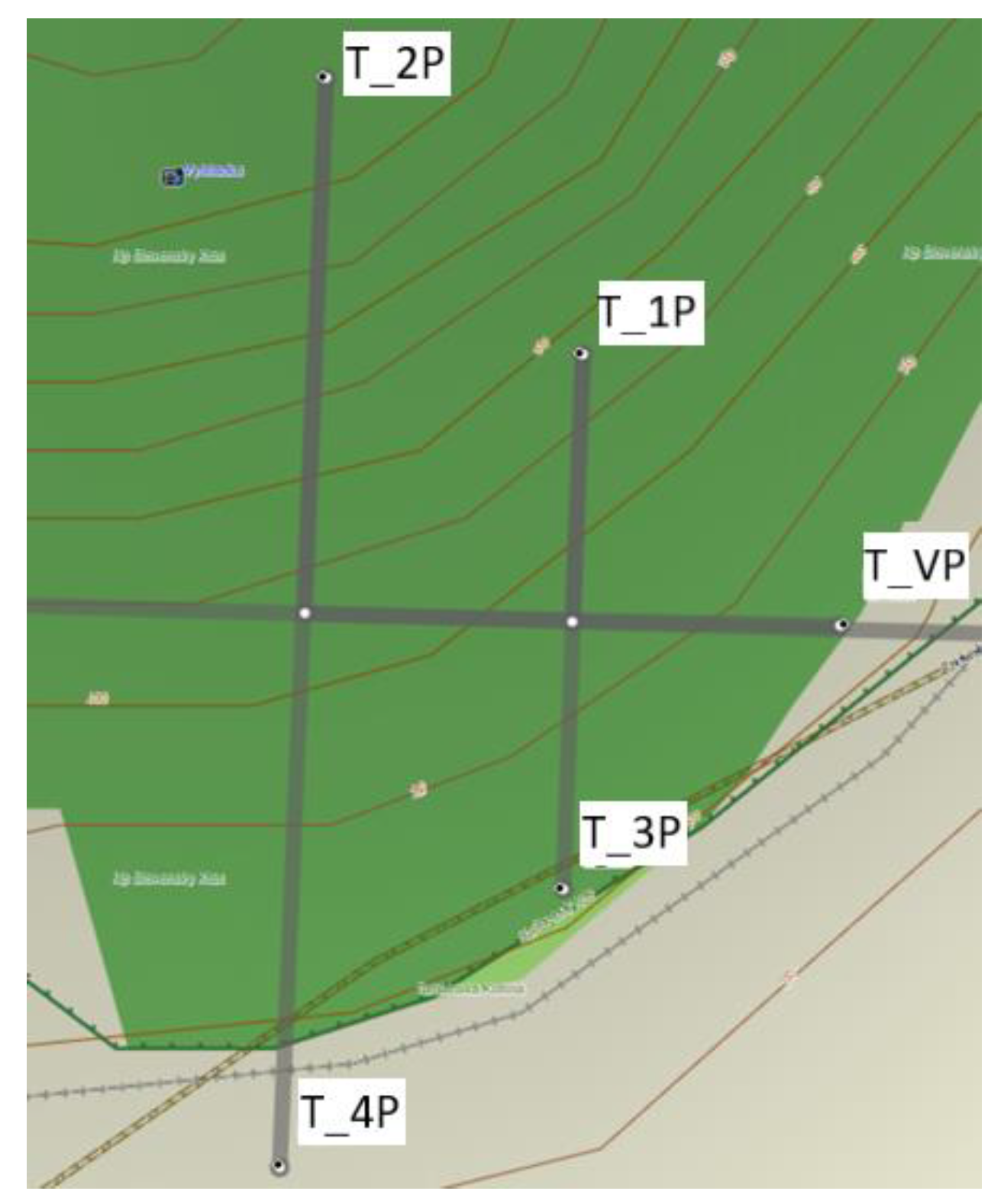
In
Figure 2, T_VP is the position of the leader of the group of UAVs, and T_iP, i = 1, 4 are the positions of the members of the group of UAVs, 1 to 4. The coordinates of the positions of the UAV group members at the end of a rectilinear flight are provided in
Table 2. The motion model of the initial flight phase of five UAVs (rectilinear flight) was created based on these assumptions. We assumed a straight flight at an altitude of 1850.0 m. The initial coordinates of the five UAVs are shown in
Table 1. When creating the flight trajectory model, we used knowledge from our previous works [
26]. We assumed a rectilinear flight throughout the line, which can be described by the equation of a line in a three-dimensional space. The line in the space is provided by two points or one point and a direction vector. Line Xk XP may be defined as follows: the line goes through the starting point
and the final point
. The endpoint coordinates are presented in
Figure 2 and
Table 2.
For the directional vector Ū
i, we express it in the form:
Then, a parametric expression of the line
has the form:
where
is the starting point of the flight trajectory,
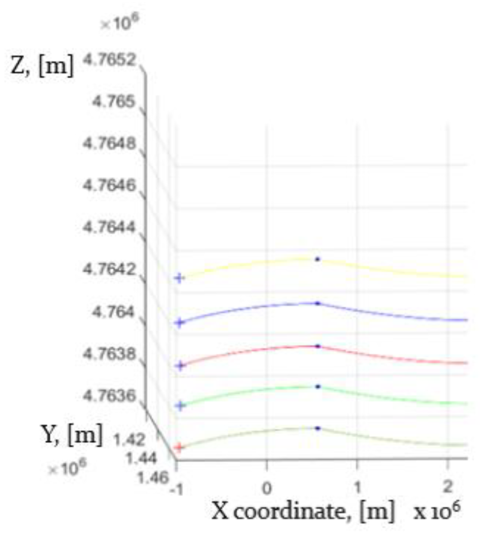
is the endpoint of a straight-line flight path, and t is the length of the step of the flight trajectory. When constructing models of five UAVs, we can choose the endpoint of the flight trajectory as desired according to the nature of the task being solved. In
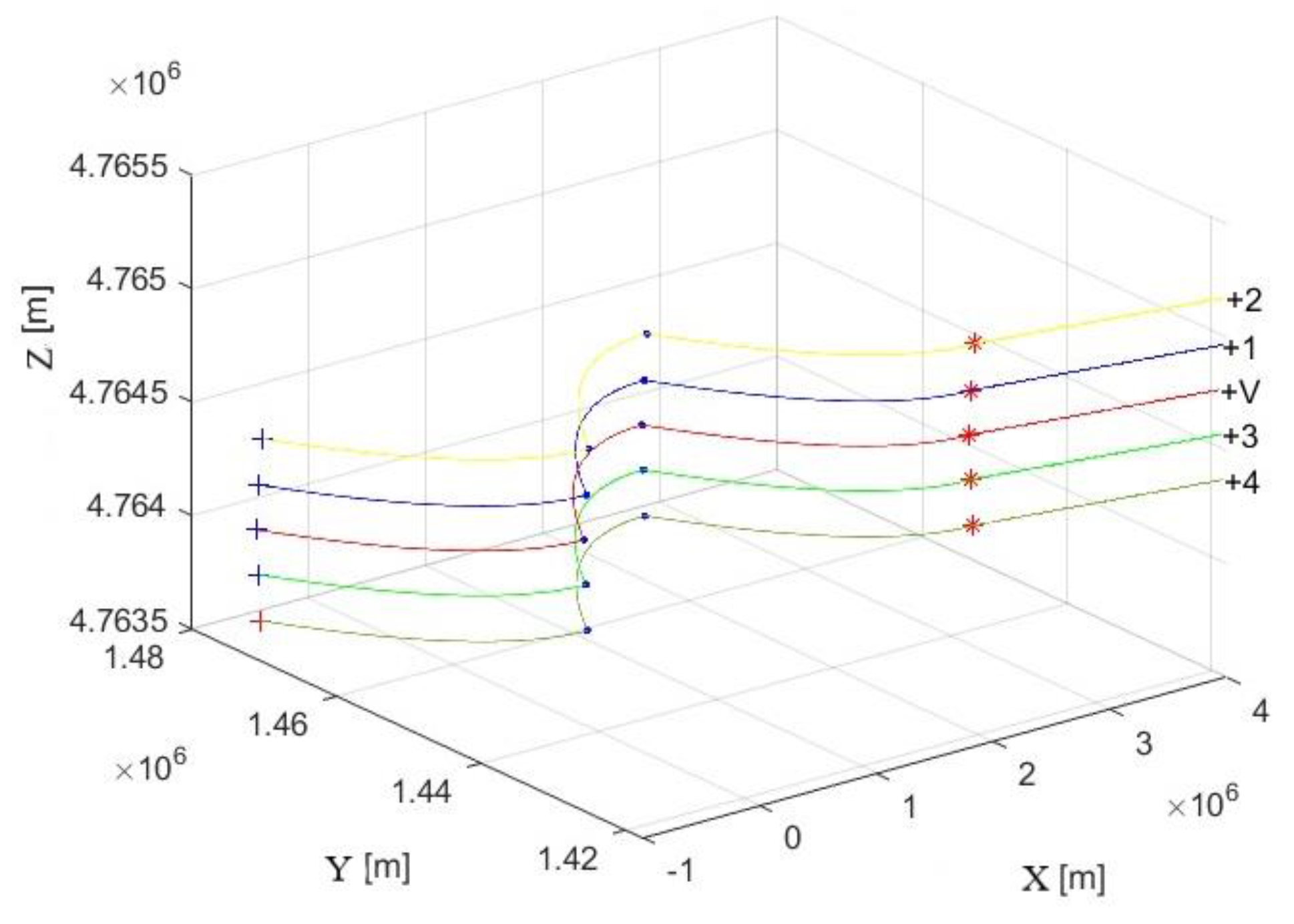
Figure 3, the initial points of the flight trajectory of individual UAVs are marked with + symbols and V or 1 to 4. The endpoints of the rectilinear flight of individual UAVs are marked with a + sign of a different color. The symbols * and ° indicate the beginning and end of the turn. Subsequently, we created models of UAV flight trajectories, formed by three turns. The models were created assuming that all UAVs fly at a constant altitude. We modeled the turns using circle shapes. The letter r denotes the radius of the circle. We assumed that the radius r must be in line with the maneuverability of the UAV.
If we have point S [x; y] = S [0; 0], it applies to all points on the circle:
If the point S is determined as
then the implicit expression of the circle is:
We express the parametric equations of this circle as follows:
When creating models of curvilinear flight trajectories of the five UAVs, we assumed that the center of rotation of the flying object was at the point
We express the parametric equations of such a circle as follows:
with Equation (6), the modeling of curvilinear flight trajectories of five UAVs was performed.
Simulation Results
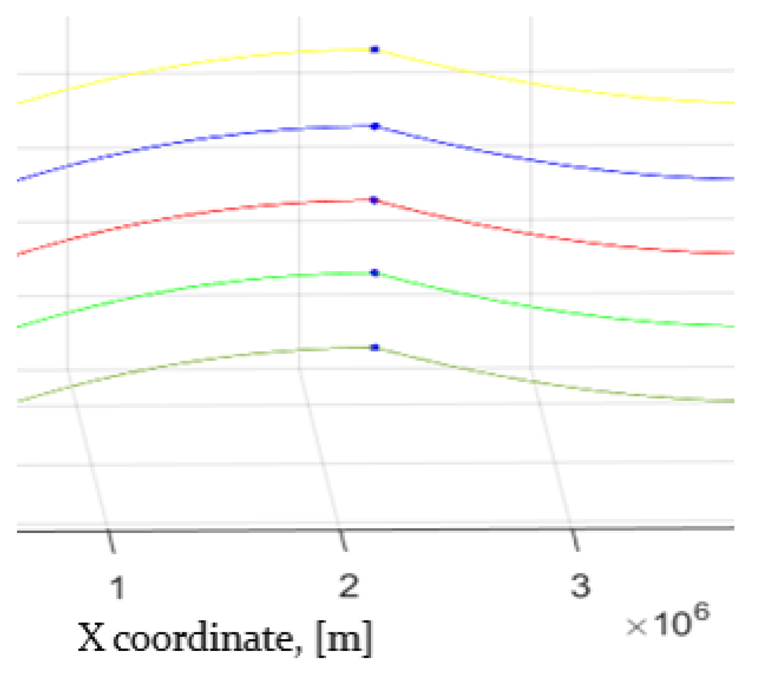
The results of the simulation of the flight trajectories of the five UAVs are shown in
Figure 3. The initial positions of the individual UAVs are marked with a + sign. The leader of the group is marked V. The other members of the group are marked with numbers 1 to 4.
The endpoints of the flight trajectories of the five UAVs are marked with + signs of different colors. From
Figure 3, it is clear that the flight trajectories of the five UAVs are composed of four parts.
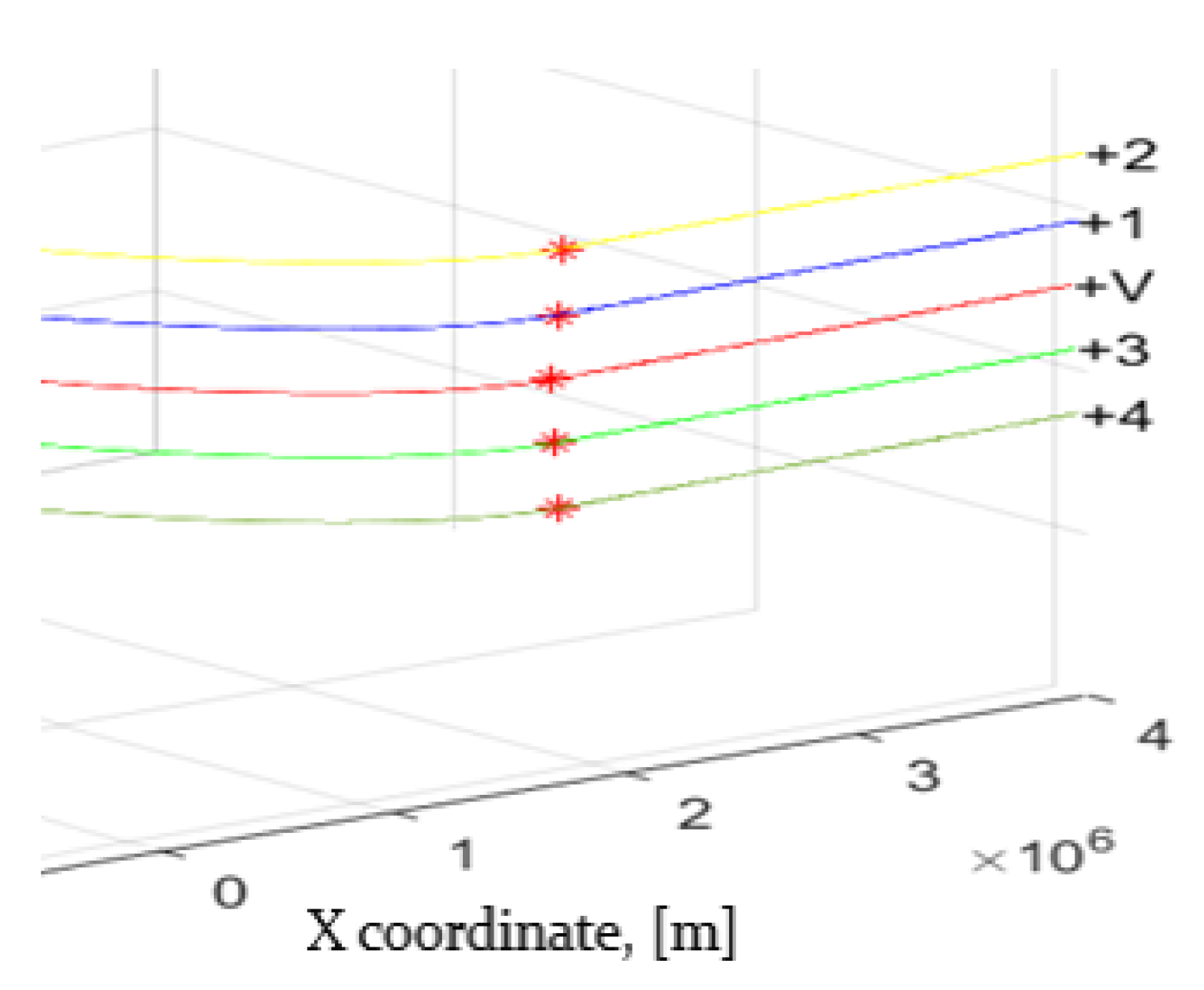
In
Figure 4, details of the simulation of the flight trajectories of the five UAVs in the first turn are shown. It is clear from the picture that the UAVs flew in a set formation and kept the specified distances between them.
A detailed simulation of the flight trajectories of the five UAVs in the second and third turns is shown in
Figure 5 and
Figure 6.
The model of the straight flight section was provided by Equations (1) and (2). The curvilinear flight model was provided by Equations (5) and (6). During the simulations, the parameters of the UAV trajectories were chosen to correspond to the flight of the General Atomics MQ-9 Reaper UAV. The flight speed was around 310 km.h−1, corresponding to 86.1 m.s−1. The height of the flight was equal to 1850.0 m due to the rugged terrain over which the UAV group was flying. The simulation results confirmed that the created models are suitable for simulating the flight of a group of five UAVs in the selected set-up. Among the main advantages of the mentioned flight model of five UAVs in a group is the model’s simplicity and the high speed of simulation.
2.2. Model of the Communication Network of a Group of UAVs
The designed model assumes that all UAVs operate in the communication network, and each UAV transmits information on its position. A prerequisite of the flight control of a UAV group is that the communication network must be synchronized. Every UAV is assigned a strictly specified time for transmitting communication messages. Designing the communication network, we started from the fact that if we know the location of a minimum of four points in space and the distances of these points from an unknown point, we can calculate the position of the unknown point. We presupposed that based on the message transmission by individual UAVs, each UAV will be able to measure distances from those users because individual users will provide times of communication message transmissions. This method of position determination is a designated telemetric method. The principle of the telemetric method is described in detail in [
27].
We assumed that all UAVs work in the communication network (see
Figure 7) and transmit in short time intervals, among other things, messages on their positions. The time of signals spreading between the UAV’s transmitter ZP_i, i = 1 to 4, and the group leader’s receiver ZP_V is directly proportional to the distance between them. Measuring the distances, d
i-v, i = 1 to 4, between UAVs ZP_i and the group leader ZP_V, it possible to determine the group leader’s location if we know the positions of the individual UAVs. The position of the group leader ZP_V against other users of communication network ZP_i, i = 1 to 4 is demonstrated in
Figure 7.
On the condition that we have identified the coordinates of individual users of the aviation communication network, ZP_i, (x
i, y
i, z
i) i = 1 to 4, and the distances, d
i-v, i = 1 to 4, of the group leader’s receiver, ZP_V, from those users, we can determine its position with the coordinates (x, y, and z). The distances, d
i-v, i = 1 to 4, of the group leader’s receiver, ZP_V, from users ZP_i, i = 1 to 4, will be determined according to the relationship:
If the user ZP_i, i = 1 to 4 sends the message at time t
i, the message will be received at time t
p. Provided that the speed of electromagnetic waves’ spreading (c) is known, the distance between the source of transmission, ZP_i, i = 1 to 4, and the group leader’s receiver, ZP_V, d
i-v, is as follows:
In reality, the calculated distance is burdened with some errors. For that reason, the distance is denoted pseudo-distance. If the time base of the group leader’s receiver, ZP_V, is shifted by an unknown time interval, Δt, then this interval can be converted to a distance, b, using the equation:
The actual distance, then, will be equal to:
where: i = 1, 2, 3, 4, d_(i-v) is the measured pseudo-distance, D
i is the actual distance, and b is the error of the distance measurement. The delay, Δt, causes a distance, D
i, measurement error due to a shift in the time bases of the UAVs and the group leader’s receiver, ZP_V.
2.3. Equations for Determining the Location of a Selected Member of a Group of UAVs
The unknown coordinates of the group leader’s receiver, ZP_V, include the unknown b, and to calculate the position ZP_V, we need four equations of the following form:
where i = 1, 2, 3, and 4.
After adjustments, we obtain:
x, y, z—position of the group leader’s receiver, ZP_V,
di-v—measured pseudo-distance from the group leader’s receiver, ZP_V, to the i-th UAV,
τi—time of the signal spreading from the i-th UAV to the group leader’s receiver, ZP_V (x, y, z),
t—time interval by which the receiver’s time base is shifted,
b—shift of the receiver’s time base converted into distance.
The position of the group leader’s receiver, ZP_V, will be expressed through 4 equations in 4 unknowns:
where d
1-v, d
2-v, d
3-v, and d
4-v are the measured pseudo-distances from ZP_
1-4 to the group leader’s receiver, ZP_V, and:
x1, y1, z1—coordinates of the UAV ZP_1,
x2, y2, z2—coordinates of the UAV ZP_2,
x3, y3, z3—coordinates of the UAV ZP_3,
x4, y4, z4—coordinates of the UAV ZP_4,
x, y, z—coordinates of the group leader’s receiver, ZP_V,
b—shift of the group leader’s receiver’s, ZP_V, time base converted to distance.
Subtraction of (16) from (13) is valid, as follows:
Subtraction of (16) from (14) is valid, and it holds that:
Subtraction of (16) from (15) is valid, as follows:
If the variable b is considered constant (the so-called factor of homogenization), then, depending on Expressions (17)–(19), a system of three equations with three unknown variables is obtained. The method of resultants of the multi-polynomials has been applied to solve the system of linear equations: x = g(b), y = g(b), z = g(b) [
27].
Then, the following applies:
If the variable “k” turns into the factor of homogenization, Jacobi’s determinant of the coordinate
x by (20)–(21) is expressed as:
In compliance with (20)–(22),
y = g (
b) is valid:
Jacobi’s determinant for the coordinate
y is expressed as:
In compliance with (20)–(22),
z = g (
b) is valid:
Jacobi’s determinant for coordinate
z is expressed as:
From Expressions (23), (27), and (31), the value of the determinants
Jx, Jy, and
Jz has been obtained. The variable equations:
x = g(
b),
y = g(
b),
z = g(
b), by applying the value of each determinant, are the results. Substituting the expression for x, y, and z into Equation (13), the quadratic function for the unknown variable b is obtained:
Solutions of the quadratic Equation (32) have two roots, b+ and b−. We calculate the coordinates of the P (x+, y+, z+) and P (x−, y−, z−). To come to the correct solution, we calculate the norm:
for (x, y, z) b− and (x, y, z) b+. If the coordinates of the receiver are fed into the coordinate reference system, the norm of the position vector will be close to the value of the radius of the Earth (Re = 6372.797 km), and this solution for P (x, y, z) will be regarded as a correct one [
27].
2.4. The Accuracy of Determining the Position of the Selected Member of the Group When Flying in a Group of UAVs
According to Equations (1)–(33), the flight of a group of five UAVs was simulated, and the accuracy of determining the position of the selected group member was evaluated. We were interested in whether using the telemetry method would make it possible to determine the position of individual UAVs and use the position determination results to control the flight of UAVs in a group. It was intended that UAVs work in the telecommunications network, as stated in the introduction of this section (see
Figure 7). The positions of the individual UAVs and the group’s flight simulation results are presented in the first section. We investigated how accurately it is possible to determine the position of the group commander using the telemetry method. First, the accuracy of the telemetry method of determining the position of the ZP_V group commander was verified, assuming that we know the positions of the individual UAVs (see
Figure 1), ZP_i, i = 1 to 4, and the distances between the individual UAVs and the group commander. The simulation results are shown in
Table 3. ZP_V are the coordinates of the group commander, and ZP_VS are the coordinates of the group commander determined by the telemetric method.
As seen from
Table 3, the simulation results confirmed that the telemetric method allows for determining the location of individual members of the group, provided that all members of the group work in the telecommunications network. A prerequisite for the exact determination of the position of, for example, the group commander, is that its receiver has the exact coordinates of the position of the other group members available. It is also necessary to know the exact values of the distance between the group commander and the individual members of the UAV group. In real life, we often encounter cases where the operation of the communication network can be intentionally disrupted by interference, or the synchronization in the communication network is unstable. This can cause errors in measuring the distance between individual members of the UAV group or determining their location coordinates. Therefore, the influence of the accuracy of the distance measurement between individual group members on the accuracy of determining the location coordinates of individual UAVs was investigated. Errors in determining the position of a member of a group of UAVs are mainly affected by the geometric configuration of the communication network users, the quality of the parameters transmitted in the FOs position report, and the network synchronization. These factors can significantly affect the accuracy of measuring the distance,
, between individual group members and the group leader. The distance measurement errors, ∆
, where i = 1, 2, 3, 4, will be modeled with a random number generator with a normal distribution. The generated random numbers will be added to the actual coordinates of the UAVs, ZP_i, i = 1 to 4. The parameters of the normalized normal distribution are E (x) = m = 0 is the mean, and the variance is V (x) = σ
2 = 1. Since we had 4 UAVs in the group, we needed 12 random number generators. The magnitude of the error of each coordinate was varied using the constant k, by which we multiplied each generated random number, where:
where: M—mean value, D—dispersion, k—non-random variable (constant), and X—random variable.
The errors were written to the row matrix for each coordinate and each user, separately:
where: i = 1, 2, 3, 4,
n is the number of simulation steps,
ΔXZP_i—row matrix of randomly generated errors of the x coordinate of user ZP_i,
ΔYZP_i—row matrix of randomly generated errors of y coordinate of user ZP_i,
ΔZZP_i—row matrix of randomly generated errors of z coordinate of user ZP_i.
Using the scalar sum operation of matrix elements 2 and matrix elements 30 to 32, we obtained new row matrices, the elements of which will represent the X, Y, and Z coordinates of each PZ_i, with errors.
where:
XZP_ic—row matrix of coordinate X of user ZP_i with error Δ xi,
YZP_ic—row matrix of coordinate Y of user ZP_i with error Δ yi,
ZZP_ic—row matrix of coordinate Z of user ZP_i with error Δ zi.
To calculate the pseudo-range between individual UAVs and the group commander, the geocentric coordinates from (2) and (13)–(16) and the coordinate errors of UAVs from matrices (33) to (35) will be used. From Relationship (7), the equation for calculating the pseudo-range, di, was obtained:
where: i = 1, 2, 3, 4 (user index), and
,
, and
are the x, y, and z coordinates of the group commander UAV.
The distance measurement error, Δdi, is as follows:
where D
i is the actual distance between individual UAVs and the group commander, and d
i is the calculated pseudo-distance between individual UAVs and the group commander.
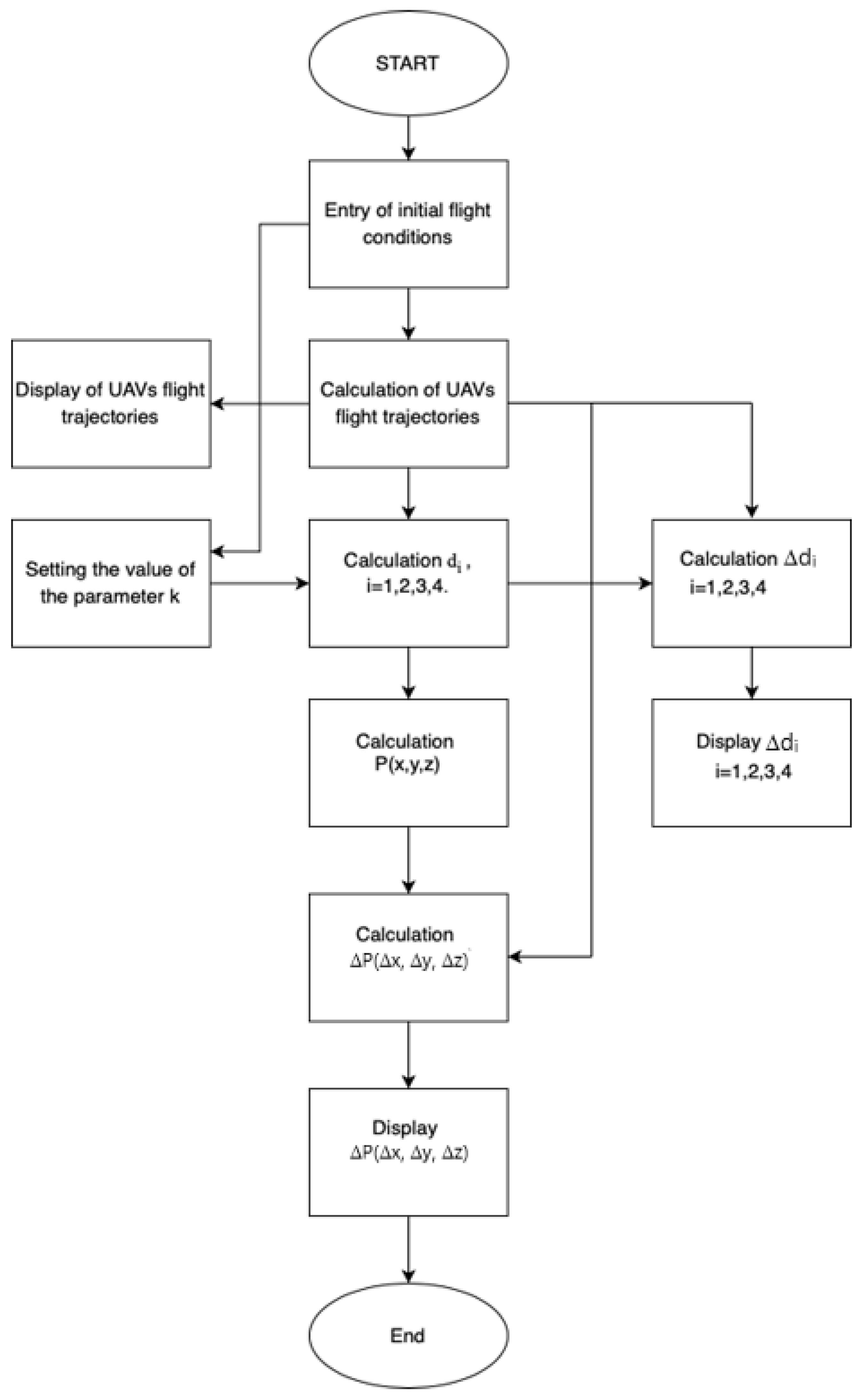
The flight simulation flow diagram of a group of UAVs and the determination of the position of the group leader is shown in
Figure 8. After entering the initial flight conditions, the flight trajectory of the group of UAVs was calculated and displayed. Subsequently, errors were generated in determining the coordinates of the four members of the group of UAVs and in measuring the distance between the individual UAVs and the group commander. The generated errors were added to the flight coordinates of the UAVs, and the position of the group leader was calculated. Based on the comparison of the calculated position of the group commander with the simulated trajectory of its flight, the errors in determining its position were determined. Then, these errors were recorded graphically.
3. Discussion and Results of the Evaluation Accuracy of Determination of the Positioning of the Group Commander
To verify the sensitivity of the proposed equations to inaccuracies in measuring the distance between individual UAVs and the group commander, we performed several simulations using the flight model of a group of UAVs, as described in the second section (see
Figure 3). The flight trajectory consisted of a straight flight and three turns. The initial coordinates of the FOs are provided in
Table 1. Initial conditions for the UAV flight models are presented in the first section. Distance measurement errors between individual UAVs and the group commander were simulated using Relations (34)–(43). The magnitude of the distance measurement inaccuracy was changed using the constant k by the Relations (34) and (35). The constant k in the range from
0.0 to 1.0 will be changed. The simulation results are shown in
Figure 9,
Figure 10,
Figure 11,
Figure 12,
Figure 13,
Figure 14,
Figure 15 and
Figure 16. Errors in determining the group commander’s coordinates are shown in blue, and errors in determining the group commander’s position are shown in red.
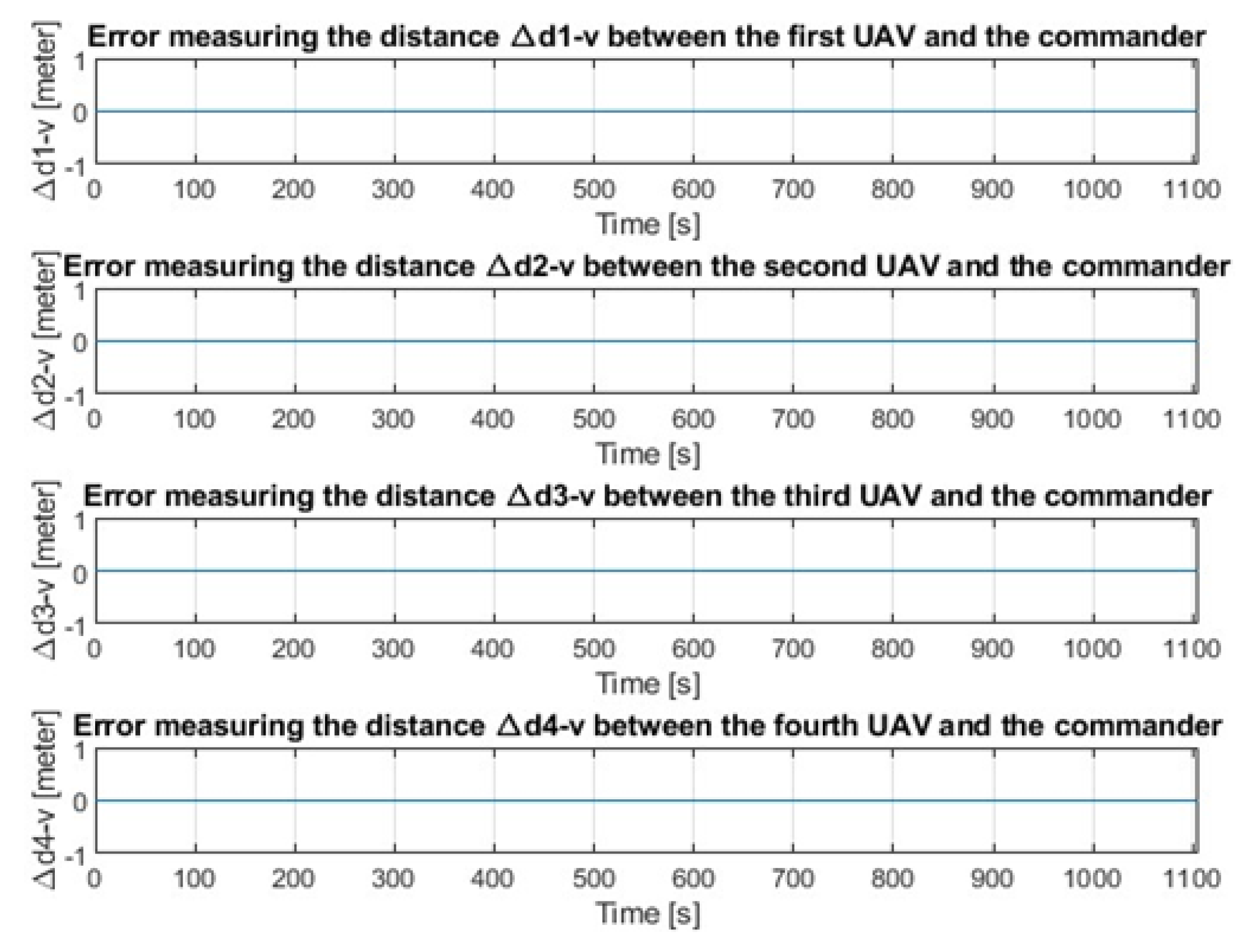
First, we checked the accuracy of determining the group commander’s position using the telemetry method during the group’s flight according to the scenario shown in
Figure 3. We assumed that we knew the exact distances between the group commander and the individual UAVs and the exact positions of the individual members of the group. In this case, the constant k was equal to zero. The simulation results are shown in
Figure 9 and
Figure 10.
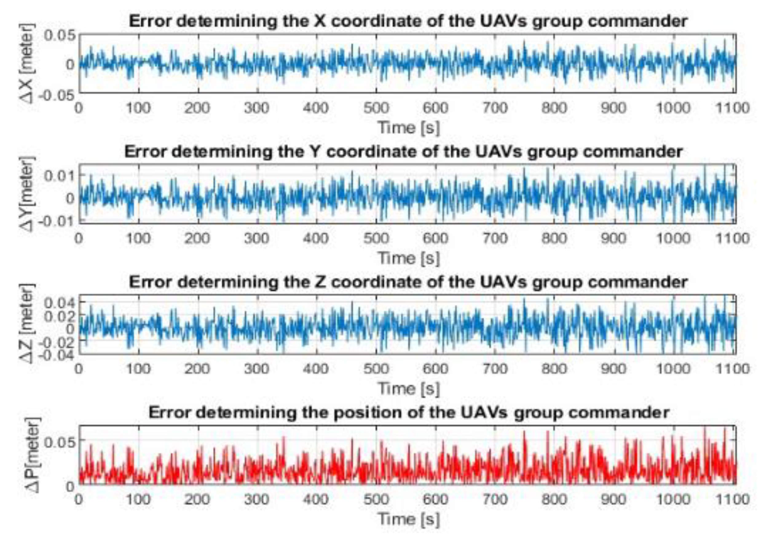
Figure 9 clearly shows that we knew the exact distances between the group commander and the individual UAVs. Therefore, the distance measurement errors were zero. In this simulation, we assumed that we knew the exact positions of the individual UAVs.
Despite this, the errors in determining the coordinates and position of the group commander were different from zero. The mean value of the error when determining the position of the group commander was equal to 0.044 m and the dispersion was equal to 2.9 m2. We consider these errors to be methodological errors of the proposed method. We investigated the effect that inaccuracies in determining the coordinates of individual UAVs and errors in measuring the distance between individual UAVs and the group commander will have on determining the position of the group commander. The constant k was equal to 0.01. Therefore, we simulated errors in determining the coordinates of individual UAVs and errors in measuring the distance between individual UAVs and the group commander by Equations (34)–(43). The coordinate and distance determination errors were random for each UAV.
The simulation results are shown in
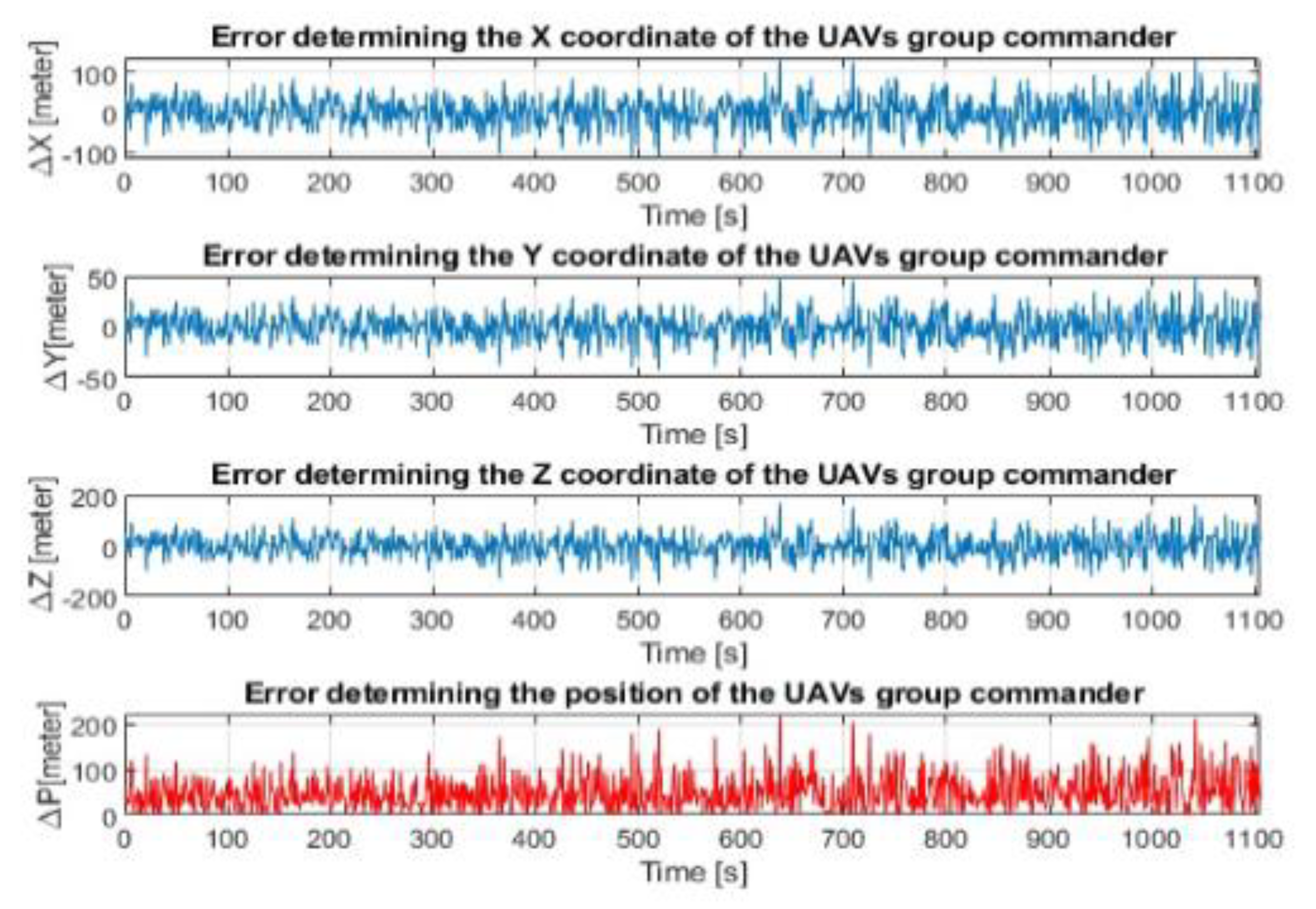
Figure 11. The simulation results clearly showed that even small errors in determining the coordinates of individual UAVs and measuring the distance between them and the group commander significantly impacted the accuracy of determining its position. This can be explained by the fact that errors in determining the position of four points in space and errors in determining the distance of these points from the position of an unknown point in space, whose position we want to calculate, have a significant impact on the calculation of the position of this unknown point. Based on the results, we investigated how the accuracy of determining the position of the group commander will change during the flight when the errors of determining the coordinates of individual UAVs are the same. Using the constant k, we varied the size of the coordinate errors. The results of these simulations are shown in
Figure 12,
Figure 13,
Figure 14,
Figure 15 and
Figure 16.
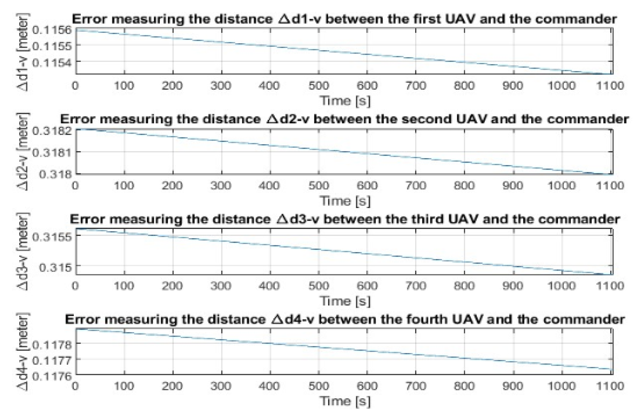
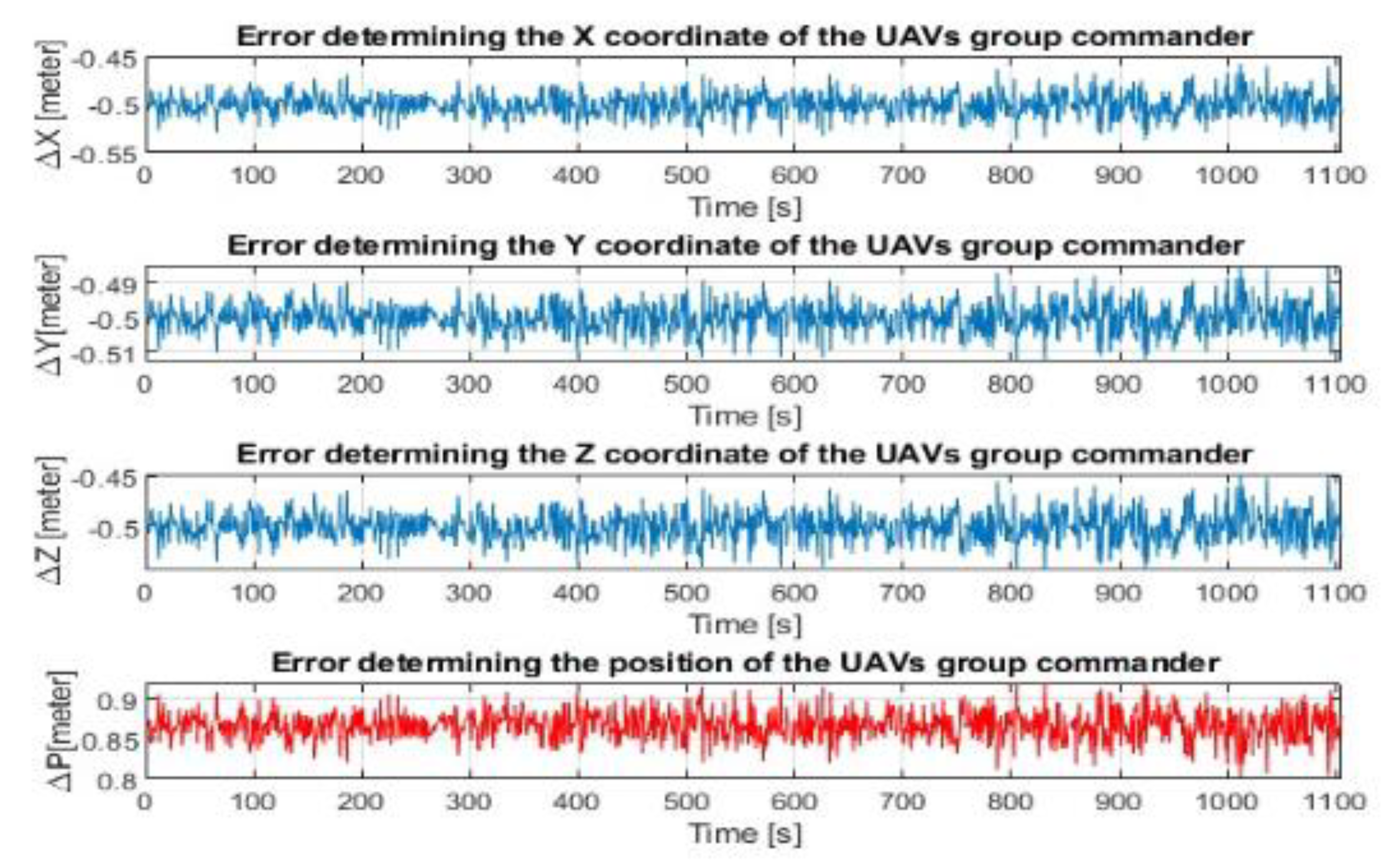
Figure 12 shows the distance measurement errors between individual UAVs and the group commander for k = 0.5. The figure shows that the distance measurement errors for k = 0.5 varied from 0.11 m to 0.31 m during the UAVs’ flight. As can be seen from
Figure 13, errors in determining the coordinates of individual UAVs and errors in measuring the distance between individual UAVs and the group commander caused errors in determining the position of the group commander’s position. For k = 0.5, the mean value of the error of determining the commander’s position was equal to 0.87 m, and the dispersion was 0.47 m
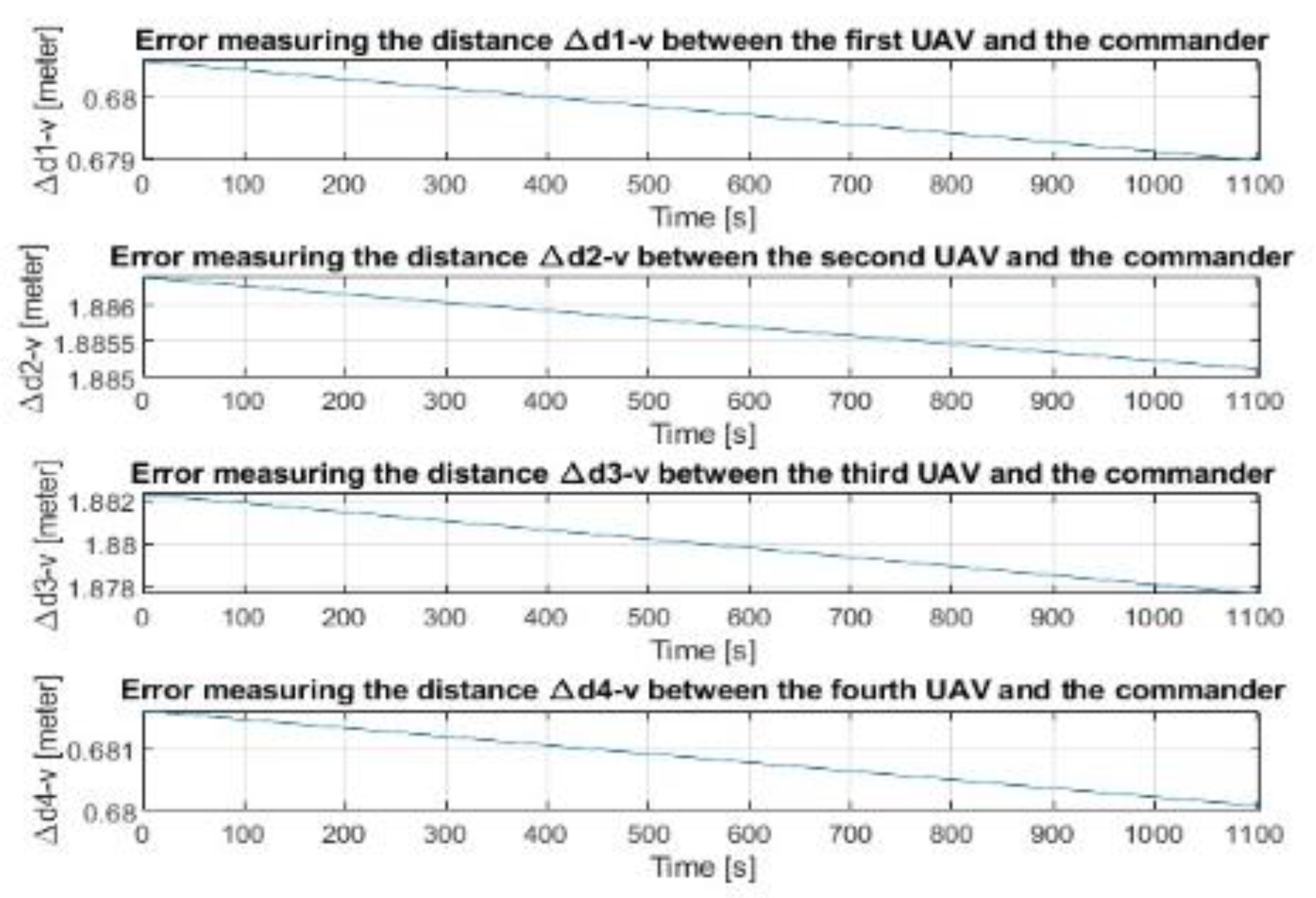
2. Next, we performed a simulation for the constant k = 3.0. In this case, the errors in measuring the distance between the individual UAVs and the group commander were from 0.67 m to 1.88 m (see
Figure 14).
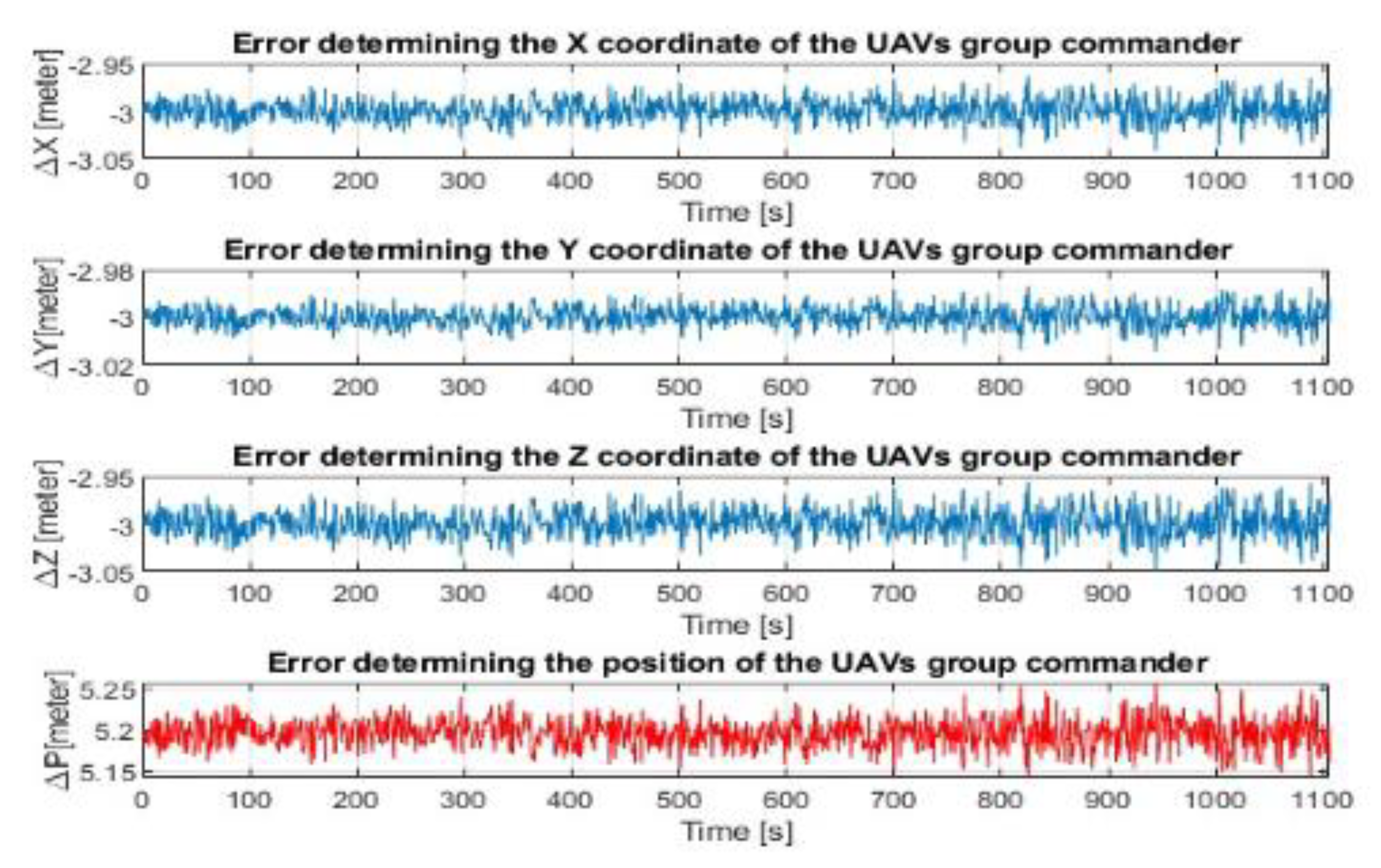
As can be seen from
Figure 15, bigger errors in determining the coordinates of individual UAVs and errors in measuring the distance between individual UAVs and the group commander caused bigger errors in determining the group commander’s position. For k = 3.0, the mean value of the error of determining the commander’s position was equal to 5.22 m, and the dispersion was 14.1 m
2.
In this way, we gradually checked the influence of the inaccuracy in determining the coordinates of individual UAVs and distance measurement errors between individual UAVs and the group commander for the constant k, equal to 0.05 to 20, which corresponded to distance measurement errors from 0.01 to 12.0 m. The simulation results are presented in
Figure 16,
Figure 17,
Figure 18 and
Figure 19.
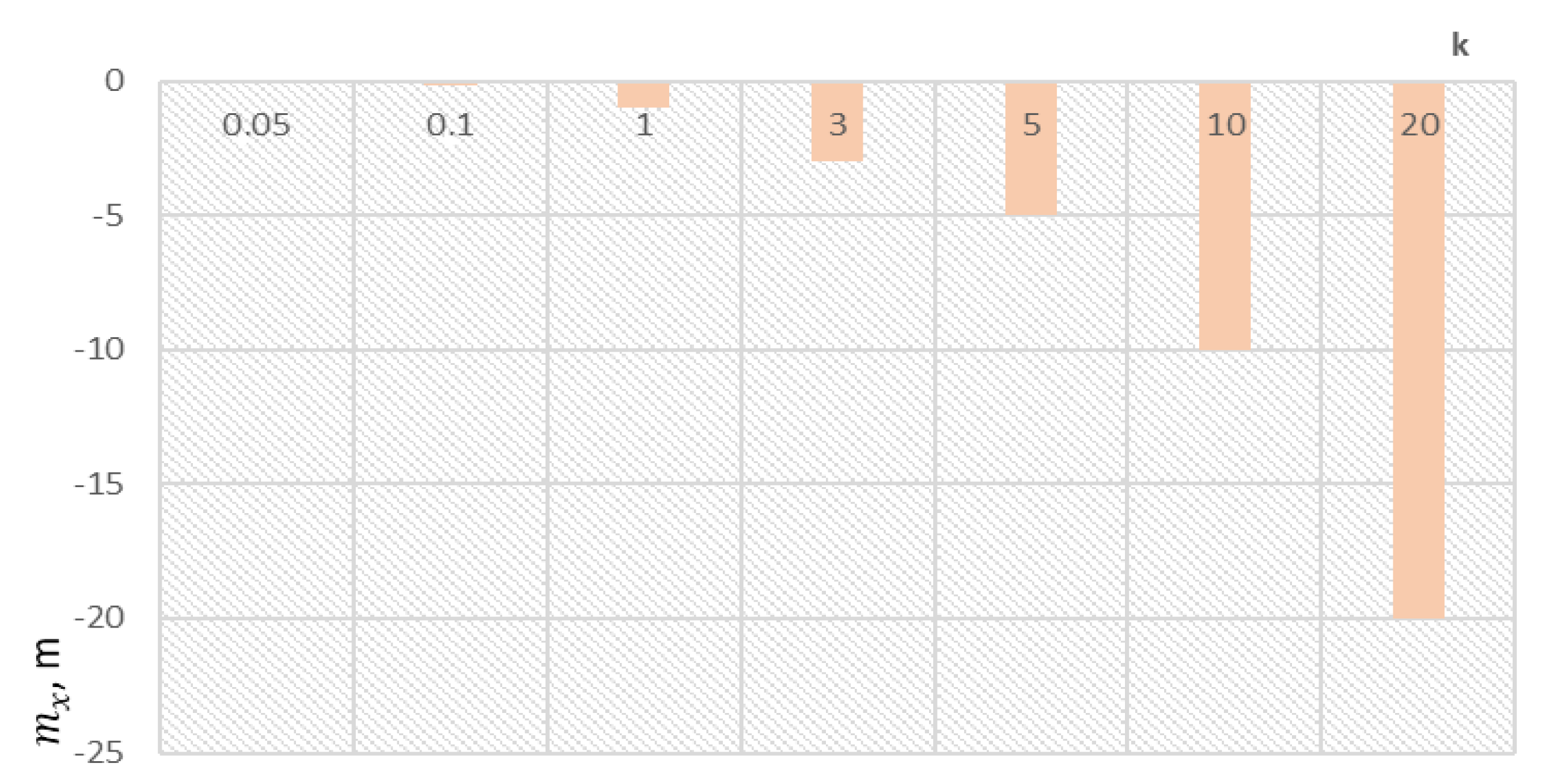
Figure 16 shows the mean values of the errors of determining the coordinate x group commander m
x for the constant k = 0.05 to 20. The mean values of the errors of determining the coordinate x group commander ranged from −0.05 m to −20.0 m.
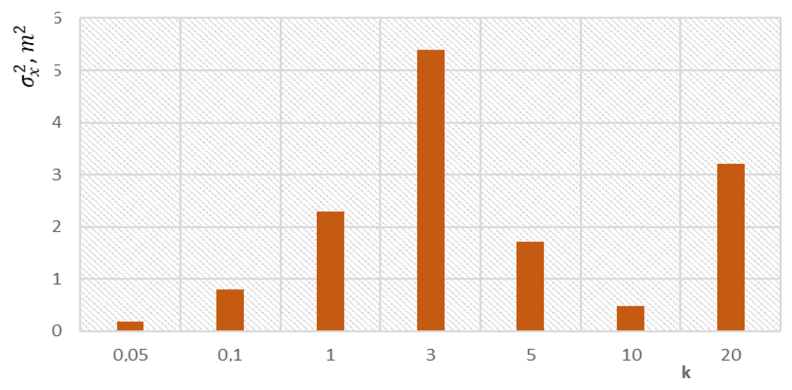
Figure 17 shows the variance of group commander x coordinate determination errors, σ
2x, for the constant k = 0.05 to 20. The group commander x coordinate determination error variance values ranged from 0.19 m
2 to 5.4 m
2.
The simulation results confirmed that when the constant k changed from 0 to 20, the errors in determining the group commander’s coordinates y and z changed in approximately the same range as the errors in determining the group commander’s coordinate x.
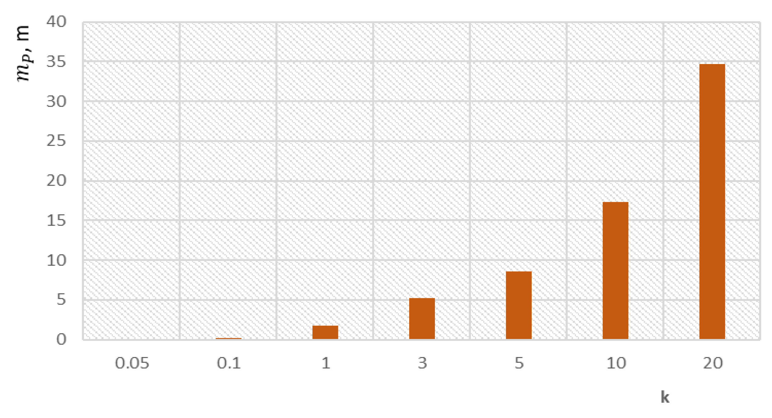
Figure 18 shows the mean values of group commander m
p position determination errors for the constant k = 0.05 to 20. The mean values of group commander position determination errors ranged from 0.11 m to 34.65 m.
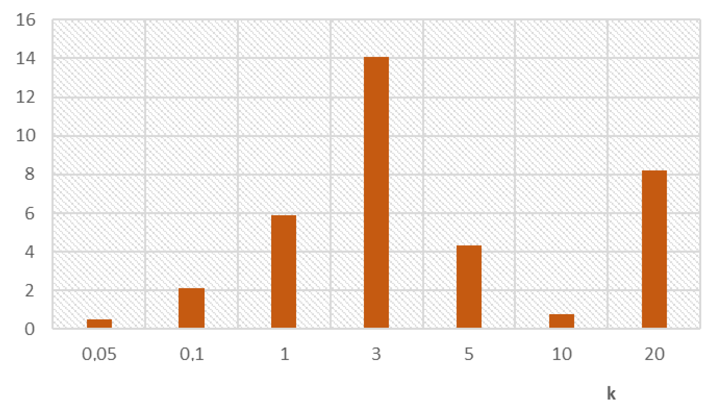
Figure 19 shows the dispersion of the group commander σ
2p positioning errors for the constant k = 0.05 to 20. The GC positioning error dispersion values ranged from 0.5 m
2 to 14.1 m
2.
The simulation results confirmed that when the constant k changed from 0 to 20, the errors of determining the coordinates y and z of the group commander changed in approximately the same range as the errors of determining the coordinate x of the group commander. The simulation results showed that if the errors in determining the coordinates of the members of the group of UAVs increased, then the errors in determining the coordinates of the group commander increased. The accuracy of determining the position of the group commander was also influenced by the accuracy of determining the distance between individual UAVs and the group commander. When the constant k was increased, the errors in determining the position of the group commander increased. Based on this, we can conclude that for accurate determination of the position of the group commander, the errors in measuring the distance between individual UAVs and the group commander must be less than 1.9 m.


