1. Introduction
An essential developmental goal for emerging economies like Thailand is the continuous enhancement of individual and household income, while addressing the pervasive issue of inequality. Achieving this goal is pivotal for the nation’s transition to a high-income level. However, this objective is complex and far from straightforward, as developmental trajectories vary among countries and are not deterministic (
Kutuk 2022). Therefore, Thailand needs a tailored approach, one that is contextually grounded, to effectively improve individual and household income.
Household income, as one of the crucial indicators of welfare, is shaped by various elements, ranging from demographic factors, employment, and education at the household level, and broader influences like economic shocks, government policies, population dynamics, and the evolution and development of various economic sectors (
Aristei and Perugini 2015;
Miles 1997;
Kalogirou and Hatzichristos 2007;
Dachin and Mosora 2012). Traditionally, the impact of sectoral shifts on income has been understood as a linear progression: starting from agriculture, moving to industrial, then to service sectors, and ultimately to knowledge-based industries (
Li 2009;
Tselios 2009). However, this linear perspective fails to fully capture the complex interactions among different sectors and their collective impact on household income. Therefore, the primary aim of this research is to provide a more comprehensive understanding of how various economic sectors influence household income.
This research is undertaken in the context of a significant economic stimulus initiative, the “digital wallet” scheme. The scheme, spearheaded by the current Thai government led by the Pheu Thai Party formed in 2023, involves issuing a one-time electronic cash incentive of 10,000 Baht (approximately USD280) to eligible citizens. This proposed economic stimulus effort, set for 2024, is designed to rejuvenate the economy, with a particular focus on benefiting the retail, service, and tourism sectors. It is expected to impact 50 million individuals and support around 2.4 million small and medium-sized enterprises (SMEs) in 2024.
1 Experts predict it could enhance the Thai economy by 1.5 to 2 percentage points, potentially leading to a growth rate of around 5%, which is higher than previous forecasts.
2One key aspect of this one-time stimulus is the scope of eligible spending. The scheme allows recipients to purchase general products, food and beverages, and consumable goods within six months of receipt. However, electronic cash in the digital wallet cannot be used for services, online purchases, alcoholic beverages, tobacco, marijuana, kratom (plant leaves used for their stimulant and pain-relieving effects), vouchers, gold, diamonds, gemstones, debt payments, education, or utility fees.
3 While the focus on essential goods and food suggests that the funds will rapidly enter the economy within a short period, there is no empirical study or explanation of how this scheme could lead to long-term benefits.
The Pheu Thai Party also claims that the scheme aims to alleviate poverty, improve welfare, and boost income at the grassroots level.
4 A significant aspect of this scheme is that the electronic cash is to be spent within the district of the recipient’s residence. This condition is intended to stimulate local economies and distribute income more evenly across the country by encouraging spending within local communities. However, it will likely be funded through government loans, amounting to around 500 billion Baht (approximately 3% of Thailand’s GDP), which has raised questions about fiscal responsibility and potential constitutional and legal issues.
5,6 Eligibility for the scheme has been a point of debate. Initially proposed to be available to every Thai citizen over the age of 16, the plan was later revised to exclude wealthy individuals.
7Considering the magnitude of this scheme, a critical question arises: will it contribute meaningfully to the long-term welfare and income of the Thai population as intended? This question is especially pertinent given that the economic sectors directly benefiting from this scheme are narrow, focused primarily on retail, wholesale, and food services. An additional question is whether this scheme is an effective way to reduce income inequality across communities in Thailand. While the scheme aims to stimulate local economies and promote equitable income distribution, its focus on specific sectors may limit its reach and effectiveness in addressing broader income disparities. Understanding the effects of various sectors on people’s income and their spatial dependencies is crucial for informing the government about potential policy improvements or necessary adjustments.
Therefore, this research is guided by two primary questions: RQ1, “what are the effects of changes in various economic sectors on average household income?” and RQ2, “what are the roles and characteristics of spatial dependencies on the effects of economic sectors and the dynamics of household income?”
To answer these questions, a spatial econometric model was employed to test the effects of 19 economic sectors comprising the Gross Provincial Product (GPP) of Thailand’s 76 provinces on the average household income in these provinces. The study utilised biannual data from 2005–2021 from the National Statistical Office of Thailand. The results of the study reveal that the sectors of agriculture, real estate, professional services, support services, and leisure showed significant direct associations with household income. Furthermore, the study discovered pronounced spatial autoregression, indicating that the income levels in one province could significantly influence nearby provinces. This finding aligns with existing literature emphasising spatial correlation.
The next section of the paper reviews literature relevant to the drivers of household income, followed by sections on data and methods, findings, a discussion, and conclusions. The study aims to provide a comprehensive understanding of the relationship between economic sectors and household income in Thailand, offering insights that could inform future economic policies and strategies.
3. Data and Method
3.1. Data
Dependent variable: In Thailand, a crucial dependent variable for assessing economic conditions is the average household income by province, as compiled by the National Statistical Office (NSO).
8 This dataset encompasses data from 2004 to 2021, covering Thailand’s 77 provinces. The NSO typically gathers this information biennially in odd-numbered years. However, an exception occurred in the early years of the dataset, with data for 2004 and 2006 collected prior to 2007. To ensure continuity and consistency in the dataset, the average household income for 2005 was imputed by averaging the incomes of 2004 and 2006. This methodology resulted in a total of eight distinct time periods, each spanning two years. The NSO defines household income broadly, including earnings from employment or self-produced goods, revenue from property, and any form of assistance received from others. This measure serves as a vital indicator for evaluating the financial health and well-being of Thai households, providing insights into regional economic disparities and trends over time. Of the 77 provinces, Bueng Kan was excluded from the analysis because it was established as a new province in 2011, resulting in incomplete data and calculations based on a different annual basis.
Independent variable: Regarding the independent variable, GPP in Thailand serves as a critical economic indicator, mirroring the concept of Gross Domestic Product (GDP) but on a provincial level. The compilation and calculation of GPP is a collaborative effort involving multiple agencies.
9 The GPP encompasses various economic parameters, including returns on primary production factors such as land rent, labour compensation, interest, and profits. It accounts for total “value added” from all economic activities within each province. The value added, a central element in GPP, represents the net output of a province, calculated as the difference between the production value (Gross Output) and the costs of intermediate goods and services (Intermediate Cost). The NSO adopts the Chain Volume Measures (CVMs) method for calculating GPP. This method, which adjusts for inflation, offers a more accurate depiction of real changes over time through a chain-linked approach.
10 The 19 economic sectors included in Thailand’s GPP are categorised into 1 agricultural, 4 industrial, and 14 service sectors, as detailed in
Appendix A.
3.2. Spatial Weight Matrix
A spatial weight matrix is a tool used in spatial analysis to represent the spatial relationships among different locations. It quantifies how much influence one location has on another, based on factors like distance, connectivity, or other relationships. This matrix is crucial for spatial econometrics, hel** to understand and model spatial dependencies and interactions.
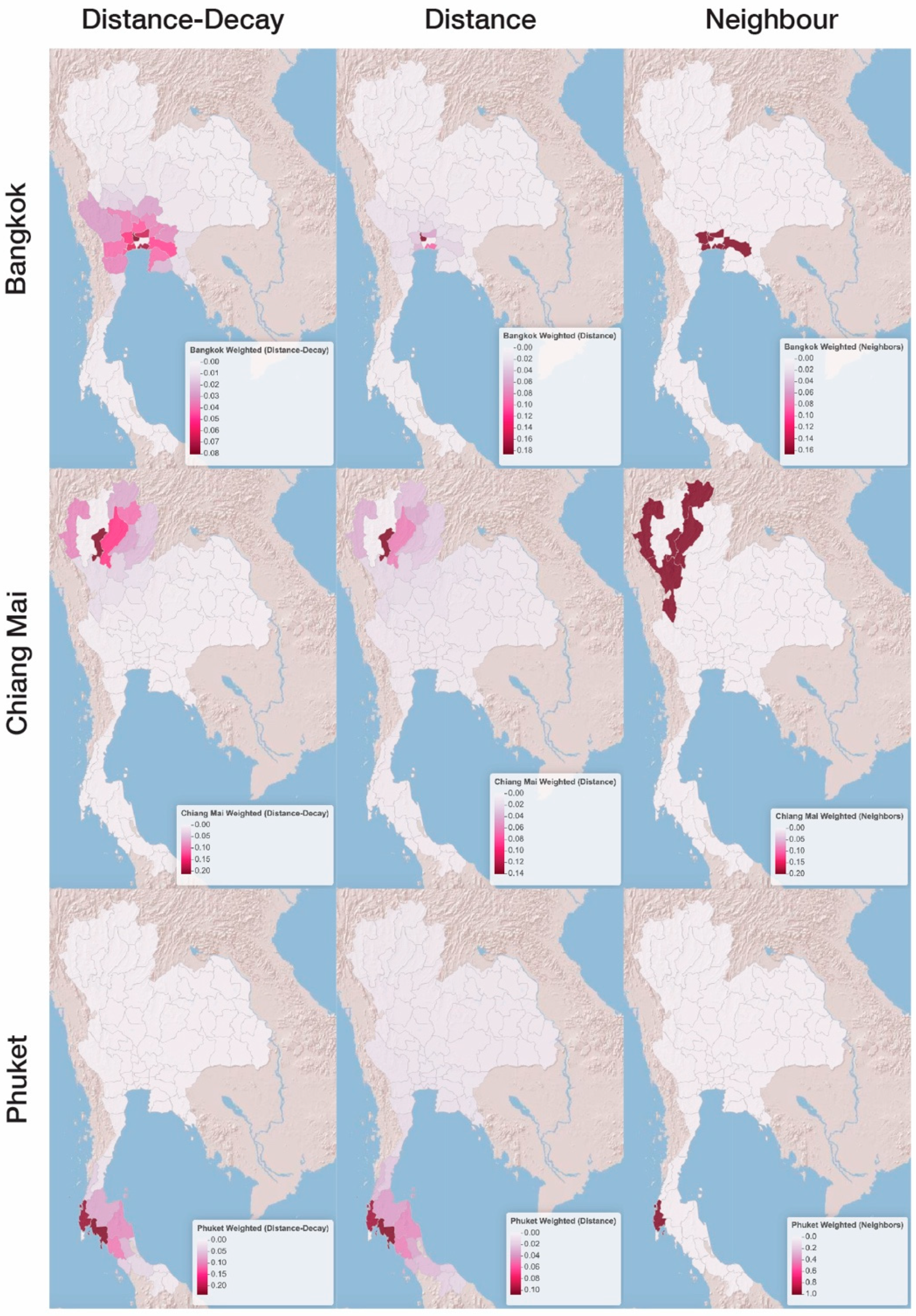
The most commonly used spatial weight matrices in spatial econometrics are the contiguity-based (neighbour) matrices, the inverse distance, and the inverse distance raised to some power or exponential distance decay matrix (
Bulty et al. 2023). The selection of spatial weight matrices is characterised by a great deal of arbitrariness, which causes a problem in inference. As the spatial weight matrix should also be theoretically grounded, this research produced the metrics based on the three methods to visually analyse and decide on the one that is most suitable. Each matrix is then row-normalised to ensure comparability.
The contiguity-based (neighbour) method is effective in accounting for provinces in close proximity, emphasising immediate spatial relationships. The inverse distance method, on the other hand, ensures coverage of the entire nation, diminishing the influence of distance but considering all regions. Conversely, the inverse distance-decay method combines the advantages of both the neighbour and inverse distance approaches. While maintaining a focus on nearby provinces, this method also accounts for more distant provinces, thus providing a more comprehensive view of spatial relationships.
The efficacy of the inverse distance-decay method, particularly in highlighting regional influences, is further corroborated by visual maps in the
Appendix A (
Figure A2). These maps display the weights of three sample provinces—Bangkok, Chiang Mai, and Phuket—and are shown in the
Appendix A. The visualisation reveals that the inverse distance-decay weights are superior in illustrating regional influence, especially in cases like Bangkok, which is surrounded by many other provinces. Therefore, in our analysis, a distance-decay parameter, denoted as α (alpha), was employed to emphasise regional influences over nationwide effects, setting α to 0.01%. This value was chosen to balance the focus between local and broader geographical Impacts, aligning with the literature that regional factors are significant in the context of economic interdependencies and regional variation.
3.3. Spatial Econometric Tests
In the field of spatial econometrics, particularly in handling panel data, several tests are conducted to determine the most appropriate model. A key test is the Hausman test, which is essential for choosing between fixed or random effects models. This test evaluates the consistency of an estimator under random effects in comparison to its efficiency under fixed effects. The Hausman test produced a chi-square statistic of 34.016 with 19 degrees of freedom, leading to a significant p-value of 0.0183. This result suggests that the fixed-effects model is more suitable for this analysis.
The Baltagi, Song, and Koh LM2 marginal test, applied using the “splm” package in R (
Millo and Piras 2012), is utilised to detect spatial lag or autoregression in the data (
Baltagi et al. 2003). Specifically, it aids in addressing RQ2 by allowing us to detect the extent to which economic outcomes in one province are potentially conditioned by those in its vicinity. The robust statistic of 27.854 and the highly significant
p-value (<0.001) from the LM2 test in our analysis provide compelling evidence that spatial dependencies are present and influential.
Lastly, the Granger causality test for the panel data, as suggested by
Dumitrescu and Hurlin (
2012), is employed to assess potential causal relationships. This test is crucial in determining whether one variable can predict another. Identifying these relationships is vital, as they significantly influence the choice of model estimation method. The panel Granger causality test is available in the “plm” package in R (
Croissant and Millo 2008). The test uncovered complex interactions between average household income and various economic sectors, exhibiting direct, inverse, and bi-directional Granger-causality relationships. A notable limitation of this analysis is the biannual frequency of household income data, necessitating its pairing with biannual sectoral GDP data. This limitation restricts the availability of figures to the year immediately preceding the year of the outcome variable. While the results are insightful, caution should be exercised in interpreting their implications due to the discontinuity in data. Nevertheless, the findings suggest potential “simultaneity” between sectoral GDP and household income, highlighting the importance of incorporating appropriate spatial econometric estimators.
3.4. Spatial Lag Model (SLM) with Fixed Effects
The Hausman test indicates the need to incorporate a fixed effect into the selected model. Additionally, the Baltagi, Song, and Koh LM2 marginal test suggests the essential inclusion of a spatial lag. Consequently, this study adopts the Spatial Lag Model (SLM) (
Bivand et al. 2021). The SLM, also known as the Spatial Autoregressive Model (SAR), is a fundamental component of spatial econometric models. It focuses on incorporating spatial dependence by including a spatially lagged dependent variable. SLM or SAR is a robust econometric model that has been insightfully used to analyze a variety of outcomes, including economic growth (
Álvarez et al. 2016;
Amidi et al. 2020), crime (
Chanci et al. 2023), COVID-19 cases (
Guliyev 2020), and pollution (
**e et al. 2019). In this model, the dependent variable for each spatial unit is regressed not only on the independent variables but also on the values of the dependent variable of nearby provinces (see Equation (1)).
where
is the dependent variable for province
at time
.
is the coefficient for the spatial lag.
is the spatial weights matrix.
is a matrix of independent variables for province
at time
.
is the province-specific fixed effect.
is the time-specific fixed effect.
represents the error term for each province at each time point.
The inclusion of temporally lagged dependent and independent variables was considered. However, this approach posed a potential risk of exacerbating multicollinearity. To address these concerns while still exploring the temporal dynamics of the data, the SLM model was adapted to include temporally lagged independent variables, resulting in SLMt. In the SLMt−1 model, sets of independent variables from previous time periods (t − 1) were used to predict outcomes in subsequent periods. For instance, in SLMt−1, sectoral Gross Provincial Product (GPP) data from 2020 were utilised to model the average household income of 2021. This approach of employing separate temporally lagged models allows for an enhanced understanding of the temporal impact of economic sectors on average household income, providing valuable insights into the temporal dimension without further complicating the model structure. Additionally, one-period temporally lagged independent variables are used as instrumental variables, a technique that is elaborated upon in the following section. This method further incorporates the temporal dimension into the model without presenting more independent variables.
3.5. Estimation of the Models
In the estimation of SLM model with fixed effects, the Maximum Likelihood (ML) method was initially considered. However, this approach was subsequently dismissed due to signs of simultaneity in the data as shown in the Granger test results. To address these concerns, the Two-Stage Least Squares (2SLS) method was employed as an alternative to ML (
Kapoor et al. 2007). The 2SLS approach is particularly adept at mitigating simultaneity issues, making it a more suitable choice for the data at hand (
Reed 2015).
In the implementation of the 2SLS method for the panel data model with fixed effects, a specific strategy was adopted for dealing with the endogenous variables, which in this case were the 19 economic sectors. The independent variables were treated as endogenous, and their one-period temporally lagged values were utilised as instrumental variables in the 2SLS method (see
Reed 2015). The Two-Stage Least Squares method for panel data with fixed effects was applied to fit all the models in this study, utilising the “splm” package in R.
3.6. Spatial Autocorrelations
Additional tests conducted to answer RQ2 include the use of Moran’s I, an index that depicts the spatial autocorrelation characteristics of average household income among provinces from 2005 to 2021. In this paper, the global Moran’s I is employed, which typically ranges between −1 and 1. A value greater than zero signifies positive autocorrelation, whereas a value less than zero indicates negative autocorrelation. This analysis was performed using the “spdep” package in R (
Bivand et al. 2015).
The global Moran’s I measure, commonly used to assess spatial autocorrelation, offers a general indication of how similar or dissimilar values are across a geographic space. However, it is limited in identifying specific local patterns, as it summarises the entire spatial distribution into a single statistic. While it can detect overall clustering of high-value and low-value areas or the juxtaposition of high and low values, it cannot discern if both types of clustering coexist. To overcome this, Local Indicators of Spatial Association (LISA) decomposes the global Moran’s I, allowing for the assessment of local spatial patterns (
Anselin 1995). LISA can identify local clusters of high values (hot spots) or low values, as well as outliers and regions that deviate from the expected spatial pattern. This method enhances the interpretation of spatial data by highlighting local clusters where similar values are geographically concentrated (HH or LL) or where contrasting values are adjacent (HL or LH), thus providing an intricate understanding of the spatial distribution of economic activities (
de Dominicis et al. 2007).
4. Findings
4.1. Descriptive Statistics and Moran’s I of Variables
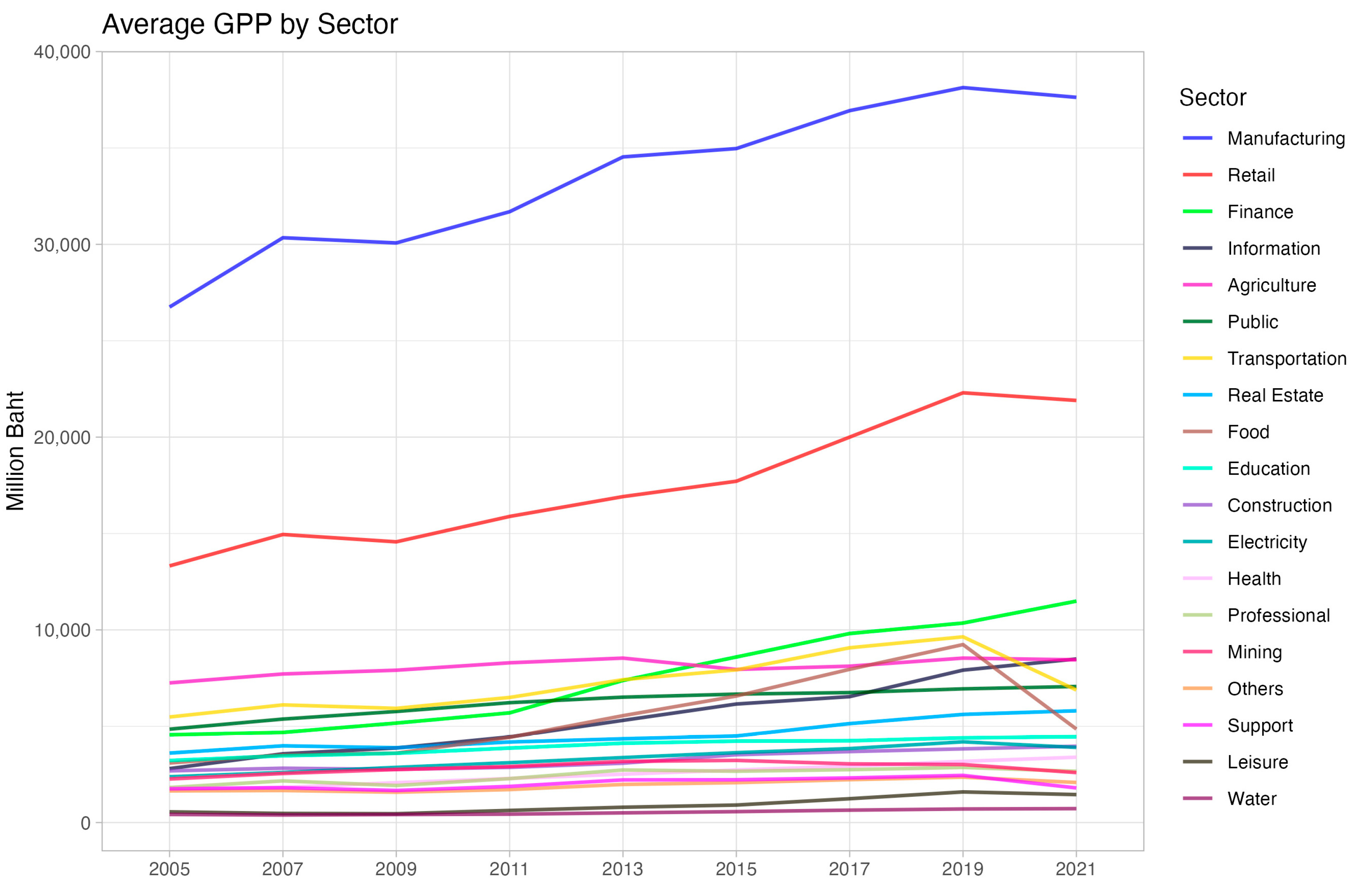
Table 1 provides a breakdown of the Gross Provincial Product (GPP) for each of the 76 provinces in Thailand, categorised by 19 economic sectors for the year 2021, with all values expressed in million Baht. The sectors range widely from agriculture to other services, with average monthly household income as a dependent variable. The manufacturing sector stands out with the highest mean GPP across the provinces (37,626 million Baht), indicating a strong presence of manufacturing activities throughout Thailand. On the opposite end, the water supply, sewerage, and waste management sector shows the lowest mean (724 million Baht), suggesting a smaller economic footprint in the provinces.
The substantial standard deviation in the retail (99,299 million Baht) and manufacturing (77,202 million Baht) sectors implies significant disparities in GPP between provinces within these sectors, possibly due to the varying presence of industrial and commercial hubs. The vast range between the minimum and maximum values across most sectors indicates a heterogeneity in economic activity, with some provinces showing very high GPP and others much lower.
The time series chart (
Figure 1) tracks the average Gross Provincial Product (GPP) of 76 provinces across 19 sectors from 2005 to 2021. It illustrates a pronounced growth trend in the manufacturing sector, which shows a steady and substantial increase over the years. The wholesale and retail sector also exhibits a significant upward trajectory, reflecting the sector’s expansion over the period. Financial and insurance alongside information and communication, though not as pronounced as manufacturing and retail, demonstrate notable growth trends, indicative of Thailand’s strengthening service economy.
However, the chart also captures the impact of the pandemic, particularly on the transportation and accommodation and food services sectors, which experienced sharp declines, reflecting global travel restrictions and reduced consumer spending in these areas during this period. The remaining sectors, including agriculture, education, and health, among others, display relatively stable trends with no significant fluctuations, suggesting resilience or steadiness in their economic output throughout the years.
Regarding the dependent variable, the Moran’s I statistics were computed (
Table 2). The analysis, underpinned by a distance-decay spatial weighted function revealed significant positive spatial autocorrelation in all observed years (2005–2021), with Moran’s I values ranging from 0.306 to 0.451 and
p-values consistently below 0.001. These results indicate that provinces with similar income levels tend to be geographically clustered. The variation in Moran’s I values across different years suggests fluctuating degrees of this clustering effect. For instance, the highest value in 2005 (0.451) points to a stronger geographic clustering of provinces with similar income levels, whereas the value in 2011 (0.306), though lower, still indicates a significant but less pronounced clustering pattern. Consequently, due to the observed autocorrelation as indicated by Moran’s I, spatial econometric modelling is deemed more appropriate than conventional econometric methods.
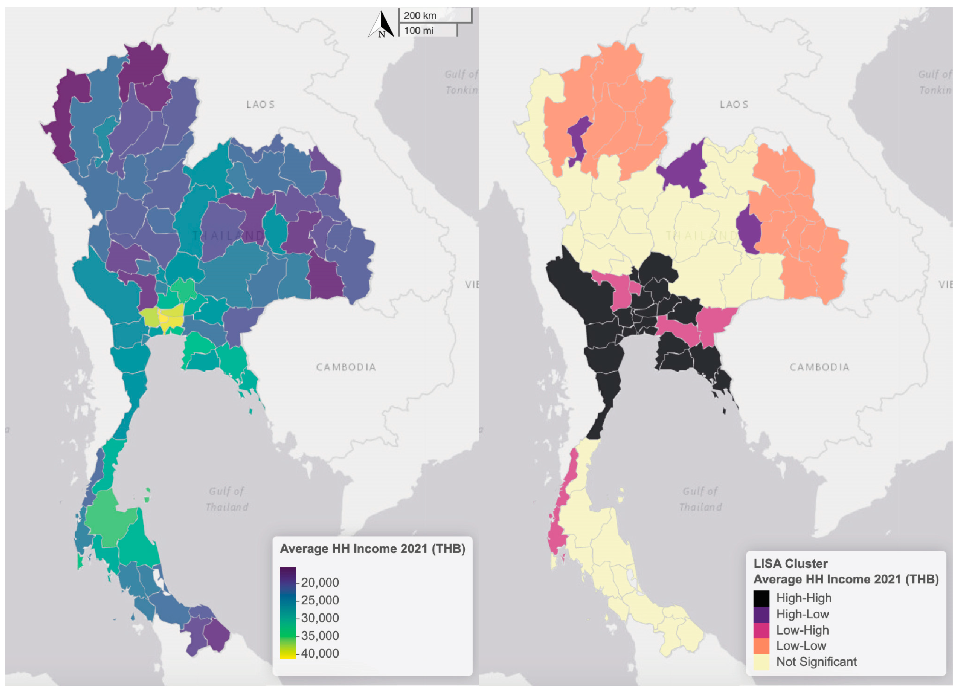
The map of Thailand displaying the average household income by province in 2021 vividly illustrates the income disparity across different regions (
Figure 2). The colour gradient represents various income levels, with lighter shades indicating higher income. Bangkok metropolitan appears as a significant area of high income, as expected due to its status as the capital and economic hub. Additionally, the Eastern region and certain parts of the Southern region also display elevated income figures. Conversely, the provinces in the Northern and Northeastern regions are broadly marked with darker shades, signifying lower average household incomes. The LISA cluster map reinforces these observations by presenting clusters of high-income provinces (H-H) in darker shades, particularly in the Bangkok metropolitan area, some Central region provinces, and the Eastern Economic Corridor. Conversely, clusters in the Northern region, as well as a large area in the Northeastern region, exhibit low-income clusters (L-L).
4.2. Results of the Spatial Econometric Models
Table 3 presents the empirical results from the application of the SLM and its lagged version, SLM
t−1. These models play a pivotal role in shedding light on the impact of sectoral economic activities on income, particularly focusing on the spatial lag effect, denoted by lambda (λ). The consistently positive and statistically significant λ values in both models (0.989 and 0.994, with
p-values < 0.001) reveal the presence of spatial spillover effects. Specifically, they indicate that household income in one province is positively correlated with the income levels in nearby provinces. This finding implies that the economic health of a region can be, in part, influenced by the financial success of its surrounding areas.
The analysis indicates that certain sectors consistently exhibit a positive correlation with average household income. Notably, the agricultural sector—which includes a range of activities from farming to fishing—displays a strong positive link with household income across both models. This relationship highlights the essential role of agriculture in sustaining rural economies and suggests that variations in agricultural output are directly connected to the economic health of provincial households. However, the earlier Granger causality tests cautions against interpreting this link as strictly predictive or causal. It likely points to a symbiotic relationship, where the success of the sector and the growth in household income are mutually reinforcing. Additionally, the real estate sector, encompassing property development and sales, shows a significant positive association in both models. This relationship may reflect the immediate economic benefits derived from real estate activities, which could suggest the sector’s impact on employment opportunities and local income levels in the short term—and the potential feedback effect of these economic conditions on the real estate sector itself.
Professional, scientific, and technical services, which range from legal and accounting to architectural services, exhibit variability in their influence on household income. They are significantly associated with the average household income in the SLM model. Administration and support services, essential to the functioning of both public and private sectors, also show a positive association with income in the SLMt−1 model. Finally, the leisure sector, which includes arts, entertainment, and recreation, presents a significant positive relationship with household income in the SLMt−1 model. This pattern indicates a short-term relationship between leisure-related economic activities and income.
While the SLM and SLMt−1 models’ results point to significant sectoral associations with household income, the simultaneity and the presence of bidirectional causality emphasise the need for careful interpretation. The two-stage least squares (2SLS) regression employed helps to address simultaneity concerns but does not eliminate them entirely. Thus, while sectoral GPP may be associated with household income, this relationship is intricate and possibly co-determined by income levels themselves.
4.3. Spatial Correlation and Regional Variations in Selected Economic Sectors
The analysis of spatial correlation in five key economic sectors significantly associated with average household income provides valuable insights into how these sectors are geographically distributed and interrelated across regions. Moran’s I was computed for two key features of each sector: the Compound Annual Growth Rate (CAGR) from 2005 to 2021, and the sectoral productivity (Gross Provincial Product, GPP) per capita in 2021 (
Table 4). The benefit of such an analysis is multifaceted; it not only highlights regions with similar growth patterns or productivity levels but also helps in identifying potential areas of spatial dependency or autocorrelation. This information is crucial for policymakers and investors aiming to understand regional economic disparities and for devising strategies to foster balanced regional development.
The Moran’s I results reveal varying degrees of spatial correlation across sectors and attributes. For example, the agriculture, forestry, and fishing sectors exhibit a significant positive spatial correlation in both CAGR (Moran’s I = 0.262, p < 0.001) and per capita productivity (Moran’s I = 0.353, p < 0.001). This suggests that regions with high growth or productivity in this sector tend to be geographically clustered. Similar patterns are observed in the real estate activities and arts, entertainment, and recreation sectors, indicating that regions with high productivity or growth in these sectors are likely to be near other regions with similar characteristics.
Conversely, sectors such as professional, scientific, and technical activities, and administrative and support service activities show no significant spatial correlation in their CAGR (Moran’s I = −0.059, p = 0.897 for the former and Moran’s I = 0.045, p = 0.059 for the latter). This suggests a more dispersed spatial distribution of growth rates across regions.
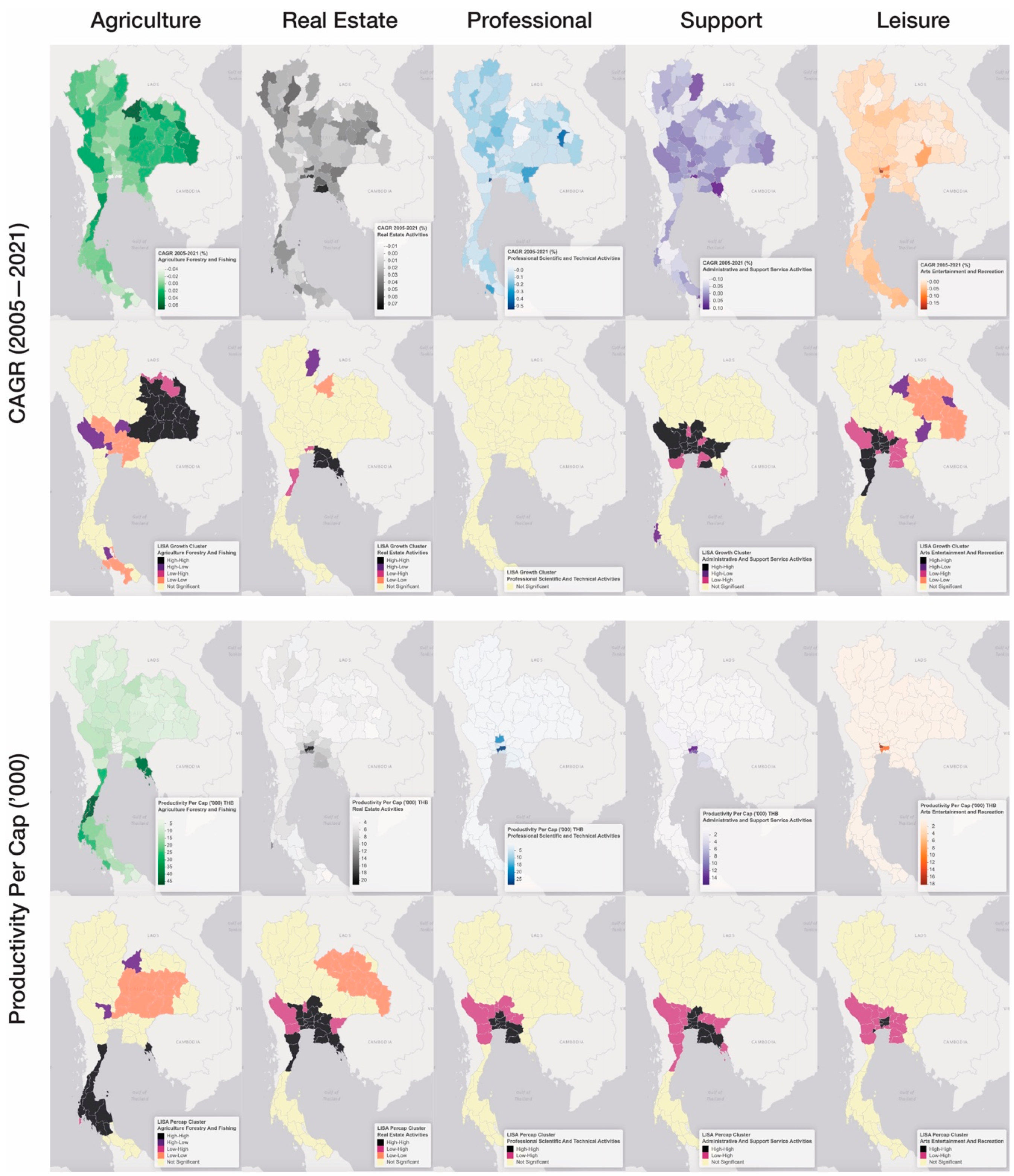
Figure 3 offers a comprehensive visual analysis of five key economic sectors in Thailand, showcasing the CAGR from 2005 to 2021, productivity per capita in 2021, and LISA cluster maps for each sector. In the
agricultural sector, the CAGR maps reveal a pronounced cluster of high growth across the entire Northeastern region, contrasting with low growth in the Central region and the deep South of Thailand. However, the productivity per capita maps indicate a starkly different scenario; the Northeastern region is identified as a low productivity cluster in agriculture, while the Southern region boasts high productivity. This contrast suggests that although the Northeastern region has seen substantial growth, it still lags in productivity, indicating a potential area for targeted development. The
real estate sector presents a strong dichotomy. The Bangkok Metropolitan area and the Eastern provinces are highlighted as regions of high productivity per capita. The Eastern region also emerges as a high-growth area, pointing to a significant divergence in growth and prosperity within the real estate sector across the country.
The professional, scientific, and technical services sector does not exhibit a clear growth pattern according to the global Moran’s I results. Nevertheless, the productivity per capita is highly concentrated in the Bangkok Metropolitan area and the Eastern region, reinforcing these areas as economic hubs for advanced services. Administrative and support service activities’ growth, while lacking spatial correlation globally, demonstrates regional high-growth clusters in the Bangkok Metropolitan area and parts of the Central and Eastern regions through the LISA Cluster maps. The pattern for productivity per capita mirrors that of professional activities, with high values clustered in Bangkok and the Eastern region. For the leisure sector, encompassing arts, entertainment, and recreation, there is a consistent concentration of high productivity per capita in Bangkok and its neighbouring provinces, Nonthaburi and Pathum Thani. The central area of Thailand is noted for the sector’s growth, whereas the Northeastern region is distinctly marked by low growth.
The LISA cluster maps presented in
Figure 3 are invaluable for discerning the distinctive characteristics and trends within Thailand’s key economic sectors. These maps highlight the spatial variability and disparities that exist, providing crucial insights that can inform and shape development policies by public sector entities.
5. Discussion and Conclusions
5.1. Discussion of the Findings
In the analysis of RQ1, “what are the effects of changes in various economic sectors on average household income?”, the study leverages the data from official sources to develop predictive models. Specifically, it employs Spatial Lag Models (SLM) and their temporally adjusted variants (SLMt−1) to delve into the effects of sectoral Gross Provincial Product (GPP) on household income. The findings indicate a potential simultaneity issue, suggesting that sectoral productivity (GPP) and average household income may be mutually reinforcing, rather than exhibiting a straightforward causal relationship.
To mitigate the simultaneity issue, a 2SLS estimator with fixed effects was employed. The analysis revealed that five sectors—agriculture, real estate, professional services, support services, and leisure—demonstrate a significant association with average household income in either or both models. Conversely, health-related sectors and other services show a negative association with average household income. These findings contribute to an expanded understanding of sectoral effects on income.
In the context of Thailand, the growth of key economic sectors is often seen as indicative of increased household income. Agriculture, for instance, employs about 30 percent of the labor force. However, this sector is characterised by relatively low income and productivity.
11 Therefore, improvements in agricultural productivity are strongly associated with an increase in average household income. Additionally, the sectors of professional, scientific, and technical activities, along with administrative and support activities, can be viewed as integral to enhancing ‘business capacity’ within a province. These sectors contribute significantly to innovation, competitive advantage, and management efficiency, all of which are closely linked to average household income.
The real estate and leisure sectors also emerge as distinct markers of increased average household income. However, there may be a bi-directional relationship at play, as these sectors are likely to benefit from the increased disposable income of the populace. The study observes no direct correlation between sectors such as retail, wholesale, and food services, and average household income, which calls for more in-depth analysis. Nonetheless, this absence of apparent relationships should be interpreted with caution due to the potential for multicollinearity in datasets of this nature.
Traditional economic theories often outline a linear transition from agriculture to industrial, service, and knowledge sectors, highlighting the transformative impact of each stage on economic development (
Kuznets 2019). This paper presents an original examination of the impact of sectoral GDP at a provincial level on household income. While this study is contextually bound to Thailand, and its applicability to other settings may be limited, it provides critical lessons for economic policy. The findings serve as an empirical foundation for strategies aimed at fostering household income growth and highlight the importance of sector-specific policies.
In response to RQ2, “what are the roles and characteristics of spatial dependencies on the effects of economic sectors and the dynamics of household income?”, the application of SLM and subsequent analysis have been instrumental. The findings demonstrate a pronounced spatial autoregression, suggesting that the household income of one province can be significantly influenced by the income levels in nearby provinces. This aligns with existing literature that emphasises spatial correlation (
Basile 2009;
Garrett et al. 2007).
The study also conducted global Moran’s I and LISA analyses on household income, growth, and GPP per capita across five key sectors. These analyses yield a two-part answer to RQ2. First, there is an apparent spatial autoregressive effect on household income, with a cluster of high-income provinces centred around the Bangkok Metropolitan region and the Eastern region, confirming a previous study (
Sajarattanochote and Poon 2009). This reflects agglomeration principles outlined in the literature, including backward linkages, innovative activity, and skilled labour pooling, which foster economic activity concentration in specific regions (
Barrios et al. 2009).
Second, sectors such as agriculture, real estate, professional and support services, and leisure, identified as potential income drivers, are predominantly clustered in this same high-income region. While existing literature discusses the convergence hypothesis, where lower-income regions gradually align with higher-income counterparts (
Chambers and Dhongde 2016;
Gebremariam et al. 2010), this study reveals a contrasting scenario in Thailand’s economic landscape. The spatial concentration of key sectors around affluent areas like Bangkok and the Eastern region signals enduring spatial inequality. However, this could be viewed through the lens of a “Kuznets-like” structural process, characterised by a shift from agricultural to industrial and service-based sectors and an initial increase in income inequality, potentially reducing over time (
Kuznets 2019). Thailand may not have reached the point where spatial inequality begins to diminish.
Despite theoretical frameworks suggesting otherwise, this study’s evidence implies that the spatial concentration of wealth and economic activities in already prosperous areas might not adequately address regional income disparities, given the low growth trajectories of these sectors across different regions. Consequently, addressing spatial inequality emerges as a critical task, necessitating collaborative efforts from both public and private sectors. The subsequent section delves deeper into strategies and recommendations, underlining the vital role of policy interventions in promoting equitable regional development.
5.2. Policy Implications
The findings of this research raise questions about the long-term effectiveness of Thailand’s digital wallet scheme. The SLM models demonstrated no direct association between the wholesale, retail, and food service sectors and household income throughout the study period. While these results do not entirely dismiss the value of the economic stimulus or downplay the importance of these sectors—which are integral to Thailand’s economy and interconnected with other sectors—they do highlight the need for a more considered approach in policymaking. The lack of direct influence between these sectors and the improvement of household income suggests that a more strategic sector- and place-based policy could be more effective.
5.2.1. Accelerating Industry Clusters and Innovation Districts
The sectoral and spatial insights from this research highlight the need for policies that specifically address these issues. The first key implication centres on accelerating economic clusters to boost household income throughout Thailand while concurrently addressing the spatial inequality identified in the study. The findings entail the crucial role of industry clusters in regional development, a strategy globally recognised for promoting economic growth (
Stimson et al. 2006).
In Thailand, economic clusters, especially in advanced manufacturing within affluent regions like the Eastern area, have been a focus for decades (
Klaitabtim 2016). However, the existing top-down approach often misses the distinctions of local realities (
Kamnuansilpa et al. 2023). This study’s insights, particularly concerning five key sectors—agriculture, real estate, professional services, support services, and leisure—suggest a more refined approach to implementing cluster policies.
Firstly, the sectors of professional, scientific, and technical services, along with administrative and support services, can be simultaneously regarded as sectors aimed at driving ‘business capacity’ in a province and are strongly associated with average household income. This research found that the improvement of business capacity is related to increased income. These findings echo the calls within Thailand for improvements in business processes, strategic planning, technical expertise, and coordination to bolster the functioning of industry clusters (
Lengwiriyakul and Jarernsiripornkul 2017;
Phochathan 2016;
Thongprasert et al. 2023;
Vanarun 2019).
This leads to the concept of “innovation districts”, a variant of small-scale economic clusters, which can significantly enhance the business capacity of enterprises and other sectors within a province. Innovation districts, leveraging the presence of universities and colleges as anchors, can facilitate public, private, and community collaborations. The integration of these educational institutions is pivotal for enhancing clusters in Thailand (
Abhinorasaeth et al. 2021;
Hansamorn et al. 2019). The existing literature also links the role of higher education institutions to regional income growth (
Liu et al. 2018;
Ramos et al. 2010;
Su and Heshmati 2013;
Teslenko et al. 2021). The innovation districts not only drive innovation and business capacity but also contribute to the vibrancy of real estate and leisure sectors (
Taecharungroj and Millington 2022).
Innovation districts in Thailand should aim to break away from a one-size-fits-all, prescriptive nationwide policy. Different regions may require distinct types of innovation districts, tailored to their unique economic landscapes and resource availability. The effectiveness of small-scale, place-based development has been recognised as crucial for regional progress in Thailand (
Moore and Donaldson 2016;
Suranartyuth 2011). These districts would provide a conducive environment for nurturing new businesses, fostering research and development, encouraging collaboration across various sectors and fostering specialisation which is important for regional growth (
Piras et al. 2012). In this context, a strategic focus on high-value agriculture as a spearhead project in innovation districts nationwide could be highly beneficial. Such a focus would leverage Thailand’s agricultural strengths, driving innovation in a sector that directly affects a large portion of the population. By integrating advanced technologies and practices into agriculture, these districts could significantly enhance household income, particularly in rural areas.
5.2.2. Improving Regulatory Framework and Province Branding
While Thailand already has various business-friendly regulations, such as tax incentives and streamlined licensing processes, these benefits have predominantly been geared towards top-down clusters in wealthier regions, with a focus on attracting large-scale investments and enhancing export opportunities (
Klaitabtim 2016). To foster more inclusive economic growth, it is essential for government policies to extend support to businesses within the five strategic sectors, especially small-scale enterprises. In addition to offering tax breaks and reducing regulatory burdens, there is a need to provide more comprehensive support, including human capital development and funding opportunities.
Another crucial aspect of place-based policy that could significantly enhance strategic sectors and income levels is the concept of “place branding” for provinces. Place branding goes beyond merely attracting tourists; it can be a powerful tool in drawing investment, entrepreneurs, and businesses to targeted provinces (
Che 2008;
Cleave et al. 2016;
Mabillard and Vuignier 2021;
Roozen et al. 2017;
Rothschild et al. 2012;
Sparvero and Chalip 2007;
Wisuchat and Taecharungroj 2022). By effectively presenting the unique business opportunities and quality of life each province offers, place branding can play a pivotal role in mitigating spatial inequality and boosting income. The combination of business and quality of life factors has been recognised as an important driver of regional growth (
Carruthers and Mulligan 2008). In Thailand, where place branding has traditionally focused on tourism, pivoting towards promoting it for business, investment, and talent attraction could direct resources to and stimulate agglomeration within key economic sectors.
5.3. Conclusions
This research offers significant insights into the dynamics of household income and spatial economic interactions in Thailand, with a focus on the effects of various economic sectors and spatial dependencies. Notably, agriculture, real estate, professional services, support services, and leisure sectors emerge as significant predictors of household income. The study’s exploration of spatial effects reveals critical spatial autocorrelation patterns. This emphasises the importance of considering regional interdependencies and variation in economic policymaking. The identification of high-income clusters around the Bangkok Metropolitan and Eastern regions, juxtaposed with the enduring spatial inequality in other areas, calls for a more progressive approach to economic development. Policy implications drawn from this research suggest alternatives to the substantial digital wallet scheme and emphasise the need to accelerate industry clusters and innovation districts, especially in less affluent regions, to promote equitable economic growth. The research advocates for a more inclusive regulatory framework and strategic use of place branding to attract investment and encourage regional development.
The limitations of this research are primarily rooted in its data constraints and the choice of econometric model. A key limitation is the temporally limited nature of the biannual average household income data spanning from 2005 to 2021. This biannual frequency restricts the temporal resolution of the analysis and may overlook subtler year-to-year variations that could offer deeper insights. Another notable limitation is the challenge posed by the often less normally distributed data, particularly with provinces like Bangkok exhibiting outsized levels compared to others. While a log transformation could have normalised the data distribution, it was not performed due to the presence of zero values in some sectors of certain provinces. Also, the potential multicollinearity among the independent variables is another limitation. The interpretation, especially regarding the size of the effects and the absence of certain relationships, should be approached with caution. Further study utilising machine learning (ML) techniques is advisable. The SLM employed in this study is a robust spatial econometric model for panel data that effectively accounts for spatial autoregressive characteristics. However, it is important to acknowledge that there are alternative models and techniques that could further enrich the analysis. These alternatives, potentially offering different perspectives and insights, could be considered in future research to overcome some of the limitations of the current study and provide a more comprehensive understanding of the phenomena.


