1. Introduction
Optical spectrometers that operate in the visible and infrared regions have become indispensable tools in our daily lives, fundamentally transforming our comprehension and interaction with a wide range of materials and substances, regardless of their physical state. This technology is extensively employed in several areas, including agriculture, energy, chemistry, materials science, and food production [
1,
2,
3,
4,
5,
6,
7,
8,
9]. The operating principle of visible–short-wave near-infrared (VIS-NIR-SWIR) spectroscopy is the transfer of energy between light and matter. This fundamental principle allows for the identification and study of different compounds by examining their distinct spectral properties. In fact, the spectral characteristics within the VIS-NIR-SWIR range are intricately linked to the vibrational modes of the functional groups found in the target substance [
2,
10]. Indeed, the vibrational modes serve as a distinctive mark, resembling a fingerprint, which enables scientists and researchers to obtain valuable information about the composition and characteristics of the substances being studied. Moreover, the non-invasive, high-resolution, and non-destructive aspects of Vis-SWNIR spectroscopy are very beneficial in plant studies [
3,
11,
12]. It enables quick assessments without causing damage to the samples, making it ideal for the real-time monitoring of plant health and nutrient levels.
Several studies used spectral analysis to investigate plants in the past [
12,
13,
14,
15,
16,
17,
18,
19,
20]. For example, Ge et al. explored the utility of VIS-NIR-SWIR as a high-throughput instrument for measuring six leaf parameters of maize plants: chlorophyll content (CHL), leaf water content (LWC), specific leaf area (SLA), nitrogen (N), phosphorus (P), and potassium (K) [
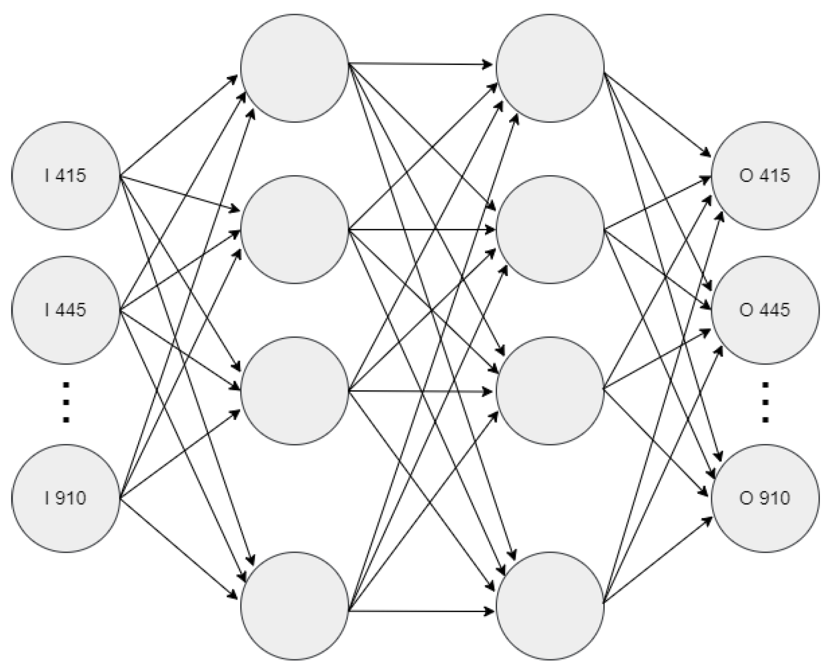
12]. To estimate leaf attributes from hyperspectral data, two multivariate modeling techniques, namely, partial least-squares regression (PLSR) and support vector regression (SVR), were used to calculate several vegetation indices. The results show that the proposed methodologies can be used to predict CHL levels but not the other leaf metrics. In 2020, ** of input data, which represents the spectrum reflectance measurements, to the matching output data, which are the reflectance values at specified wavelengths. The MLP model, which is designed for feedforward operation, adeptly captures intricate connections between the input and output data, facilitating accurate spectrum analysis and predictions. On the other hand, the weights of these connections are modified during the training process. Each neuron’s output is multiplied by the connection weight, then undergoes a rectified linear unit (ReLU) activation function and is summed with the outputs of other linked neurons. In this case, a ReLU function was selected because of its reduced training time and straightforward integration into embedded devices.
Tiny machine learning (TinyML) is a revolutionary branch of artificial intelligence that enables the execution of ML models on low-power devices, like MCUs. This breakthrough technology empowers the implementation of machine learning models for sensor data analysis directly on the device, resulting in lower power consumption and feasible deployment on battery-powered devices. The benefits of TinyML are manifold: local data processing minimizes the latency, enhancing the efficiency and expediting decision-making without the need for information transfer to a server. Moreover, reduced power consumption is critical for battery-constrained devices, while local data storage heightens the security by mitigating risks associated with information transfer. The implementation process typically commences with training the model on a higher-power computer using TensorFlow, followed by optimization with TensorFlow Lite to reduce the size and complexity. The model is then adapted to the MCU’s capabilities, and necessary code is written to load and run the model on the device, undergoing tests and performance adjustments as needed.
In this work, the perceptron training process was carried out using the TensorFlow library. The main objective of this implementation was the subsequent integration of the model in an embedded system to have the data adjusted in real-time. This optimization process is achieved through the adaptation of the model to the tiny machine learning framework, which allows for its efficient implementation on an MCU with limited resources.
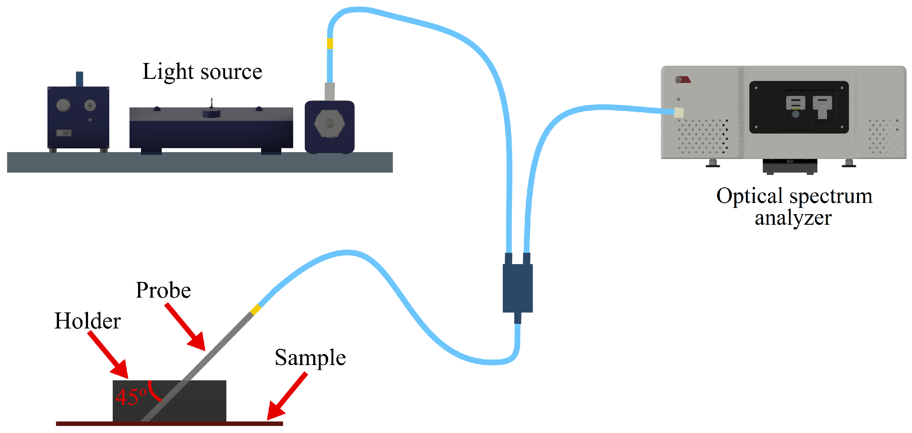
2.6. Measurement of Reflectance Using an Optical Spectrum Analyzer (OSA)
The experimental setup illustrated in
Figure 6 was employed to obtain the reflectance spectrum of colored paper sheets with different colors. This setup employed a laser-controlled plasma-type white light source (Energetiq EQ-99-FC, Wilmington, MA, USA) that emitted between 190 and 2500 nm, and an optical spectrum analyzer (OSA) (Yokogawa, AQ6373, Tokyo, Japan). Both instruments in this scenario were connected using a fiber optic probe (Ocean Optics, QR200-7-UV-VIS), which enabled the measurement of the reflectance of the sample being analyzed. As depicted in
Figure 6, the probe was strategically positioned at a 45° angle to mitigate the impact of undesirable reflections that might compromise the measurement accuracy. This orientation served the dual purpose of not only minimizing unwanted reflections but also preventing incident light from reflecting directly back toward the light source. To ensure that the measurement was always taken in the same position, i.e., at the same distance between the probe and the sample, a holder was employed. This holder was allowed for securing the position of the probe with a screw.
The OSA measurements were conducted using a linear scale with a precision of 5 nm, covering a wavelength range of 350 nm to 980 nm with increments of 0.31 nm. The initial phase of the experiment entailed capturing diffuse reflectance spectra spanning from 350 nm to 980 nm. This was achieved by utilizing a certified reflectance standard, specifically the USRS-99-010 model from Labsphere (Hewlett Packard, Palo Alto, CA, USA). This accessory helped to calibrate the white color, thereby guaranteeing the consistency and accuracy of measurements. Its function was to emulate an ideal target with nearly perfect reflectance, facilitating precise and reliable data collection throughout the experiment. Through spectral analysis of this reference sample, we established a standard against which the reflectance characteristics of other materials could be evaluated. This comparison was crucial to ensure precise and uniform measurements across all samples. By employing a reference sample, we could compensate for variations in the measurement configuration, such as fluctuations in the light intensity or sensor sensitivity, ensuring the successful normalization of the collected data. Subsequently, a series of colored paper sheet samples, with each one displaying a distinct color, were subjected to experimentation utilizing the aforementioned setup to acquire the reflectance spectrum for each colored paper sample. The selected colors were red (C01), orange (C02), yellow (C03), fuchsia (C04), violet (C05), dark blue (C06), light blue (C07), dark green (C08), and light green (C09).
3. Results and Discussions
3.1. Assembly and Manufacturing
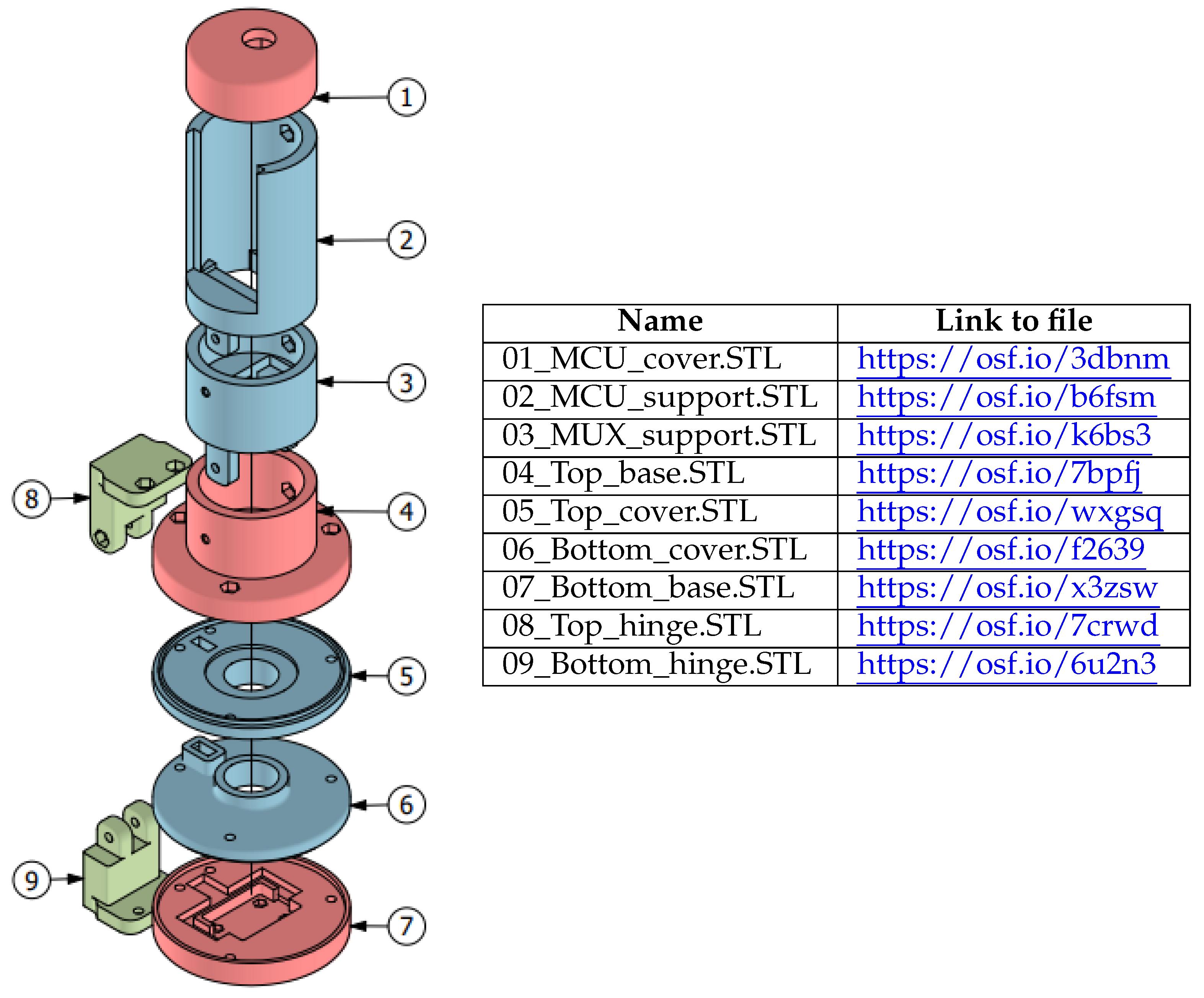
First, each element of the suggested affordable spectrometer was constructed utilizing the 3D-printing technique, specifically employing the Creality Ender 5 printer. Although polylactic acid (PLA) is a suitable material for this purpose, acrylonitrile styrene acrylate (ASA) is advised due to its superior mechanical strength and ability to protect against UV radiation. Subsequently, the assembly of all components was executed following the instructions outlined in
Section 2.2, following the assembly of the mechanical components. M3 screws and safety nuts were utilized to ensure secure assembly and prevent misalignment during operation. Additionally, two 30 mm watch glasses can be used to hide the sensors for added protection against dust ingress and facilitate cleaning. The mechanical design has space to accommodate them. The electronic system described in
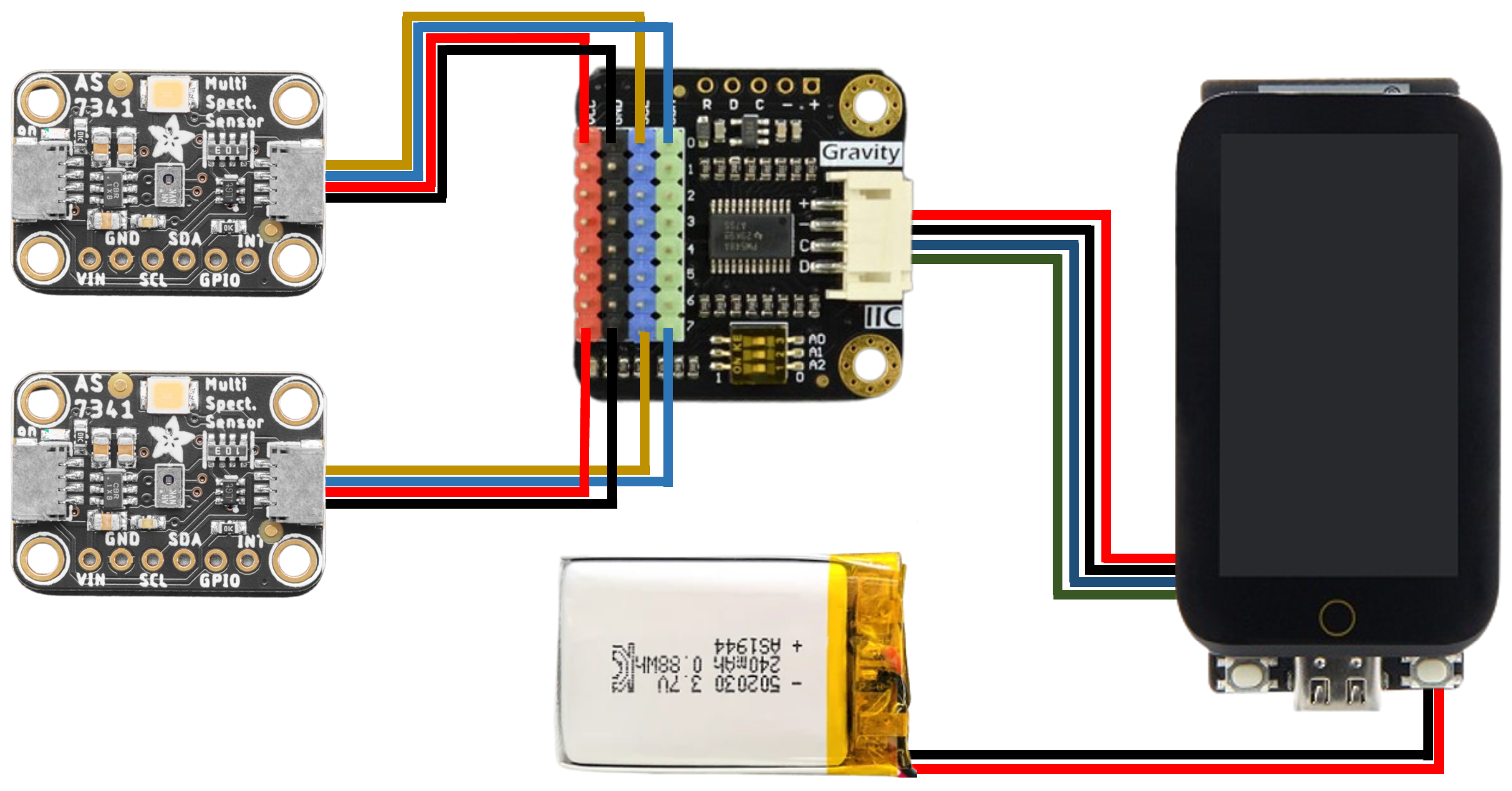
Section 2.3 was implemented in a manner that ensured optimal sensor placement to prevent any errors. An essential aspect was to ensure that each component was properly fixed to prevent any movement, as this could lead to measurement inaccuracies. Therefore, it was crucial to align the size of the mechanical components with the specific shape of each electronic element. Conversely, the software responsible for acquiring, storing, and processing data was installed in the MCU. As stated in
Section 2.5, this software incorporates a TinyML model.
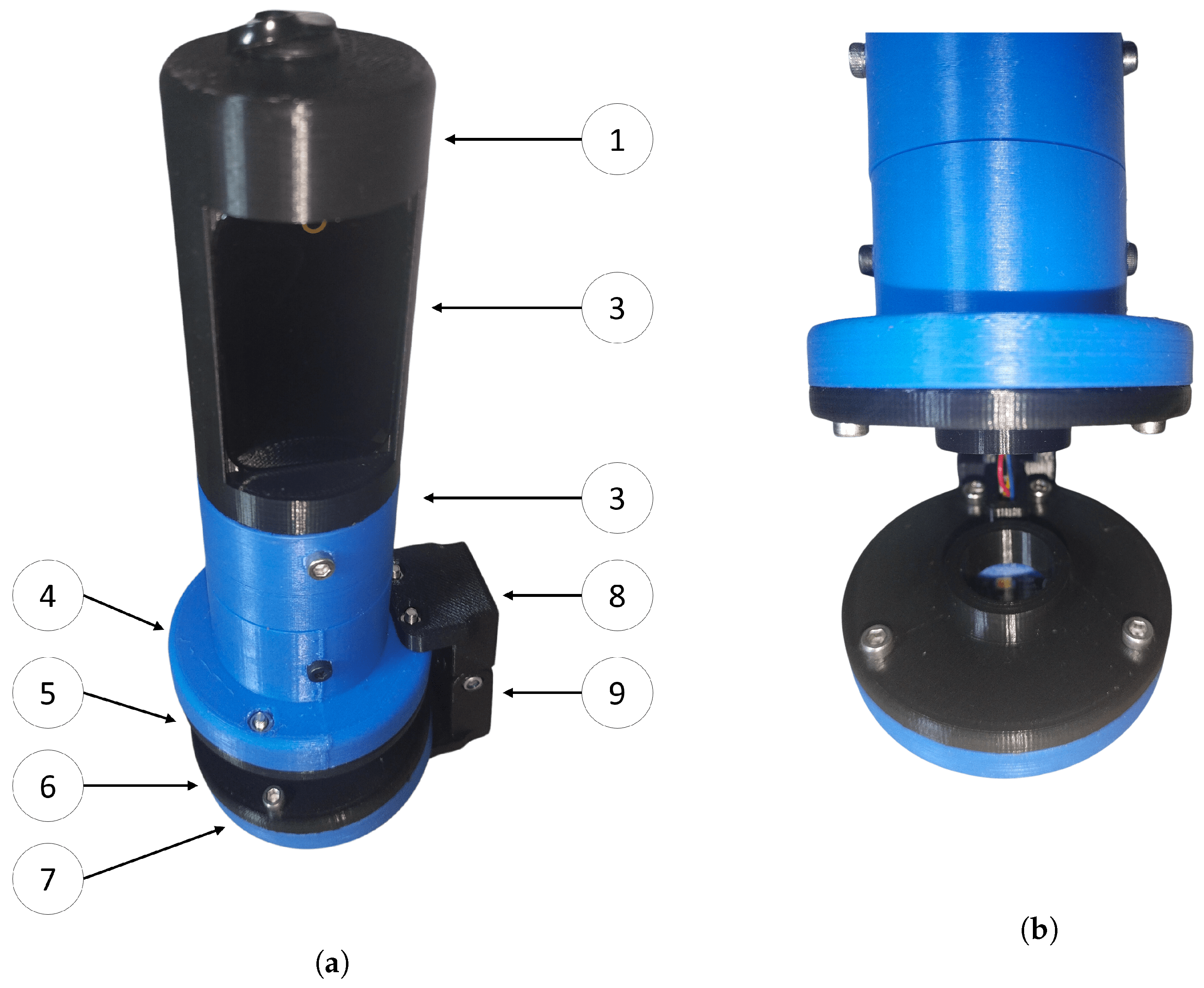
Figure 7a shows a picture of the entire view of the proposed spectrometer, and each component was sequentially labeled according to the diagram presented in
Figure 2 to facilitate their identification.
Figure 7b displays an image depicting the specific region of the device where the samples to be analyzed are positioned. The construction and integration of an affordable spectrometer was accomplished, demonstrating its user-friendly nature and suitability for use in external laboratory settings.
3.2. Model Selection and Training Error
As previously stated, the calibration dataset was drawn from the data acquired using the color checker [
33], which consisted of 24 patches with known reflectance curves, and the raw data taken from each of the sensors, considering the potential variances that may exist between them.
Table 1 presents a summary of the training for the upper sensor. A total of 16 different MLPs were trained, varying the number of layers and the number of neurons in each of the hidden layers. Given the limited amount of data, each neural network was trained five times, and the error was averaged to ensure stability. The metrics used were the mean absolute error (MAE) and total P. The total P refers to the total number of parameters in the model, in this case, the parameters were the weights and biases used to connect the neurons. The number of parameters is important as it affects the size and complexity of the model. A model with many parameters can be more accurate but may also be more challenging to train and might require more training data. In our case, it would also imply more complexity in deploying it on the embedded system. According to the findings presented in
Table 1, the model that utilized two hidden layers with 64 neurons in each layer was chosen since the inclusion of a third layer did not result in a substantial enhancement in performance. Conversely, the inclusion of a third hidden layer resulted in an almost double increase in the value of the total P metric compared with the scenario when only two hidden layers were employed. Therefore, the model would become more complex and robust, thereby increasing the difficulty of its integration into the embedded system. Furthermore, it is evident that the inclusion of a fourth hidden layer negatively impacted the outcomes, which was a phenomenon that might be attributed to limited available data.
All the conducted training sessions involved a rigorous execution process spanning 1000 epochs, each with a modest batch size of 3, while ensuring data diversity through the strategic utilization of the "shuffle" option. In the neural network architecture, only the bias was implemented in the initial layer, while the loss function was carefully designated as the mean absolute error (MAE), indicating a robust approach to error measurement. Notably, these intensive training operations were seamlessly orchestrated within the user-friendly Google Colab platform and were consistently completed within a highly efficient time frame, with no instance surpassing the 200 s mark. Both tools used have an open-source license that allows users to utilize, modify, and redistribute the software without any restrictions.
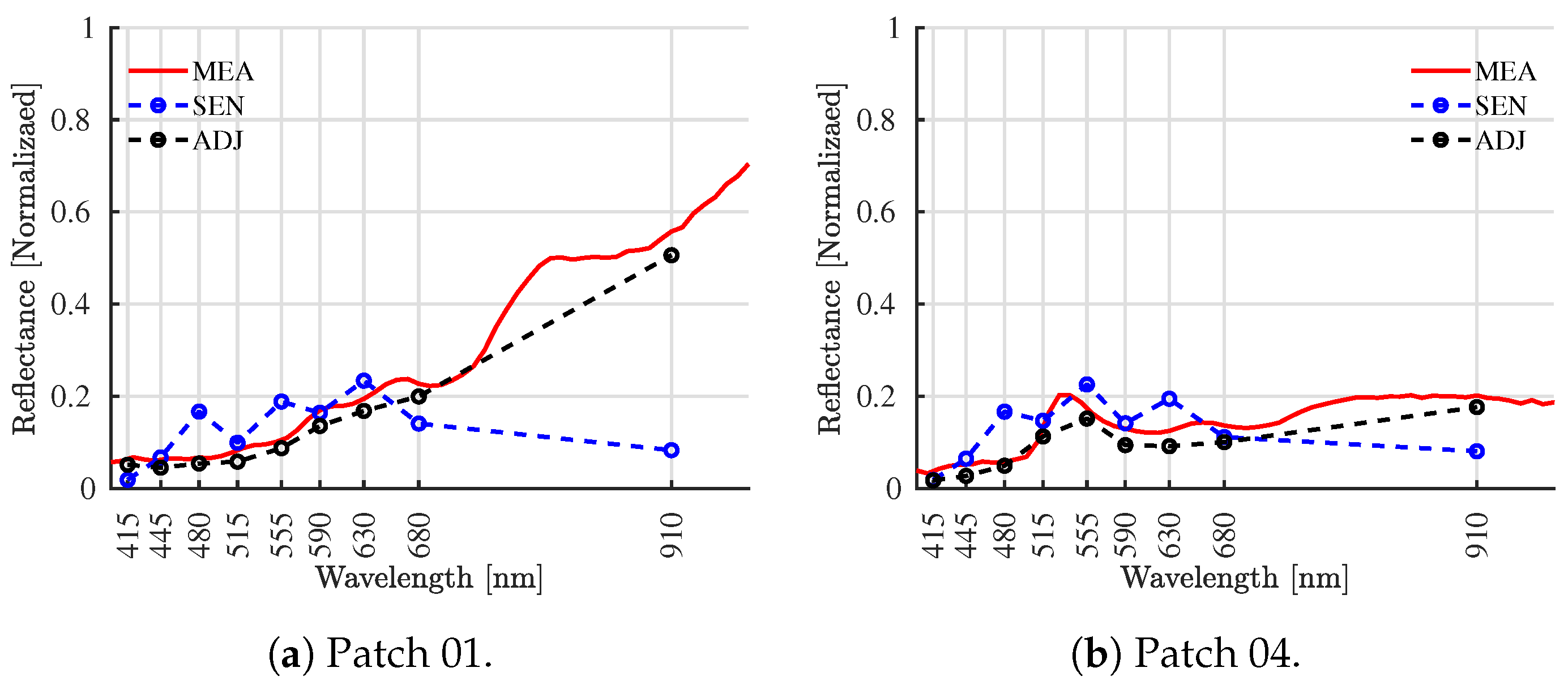
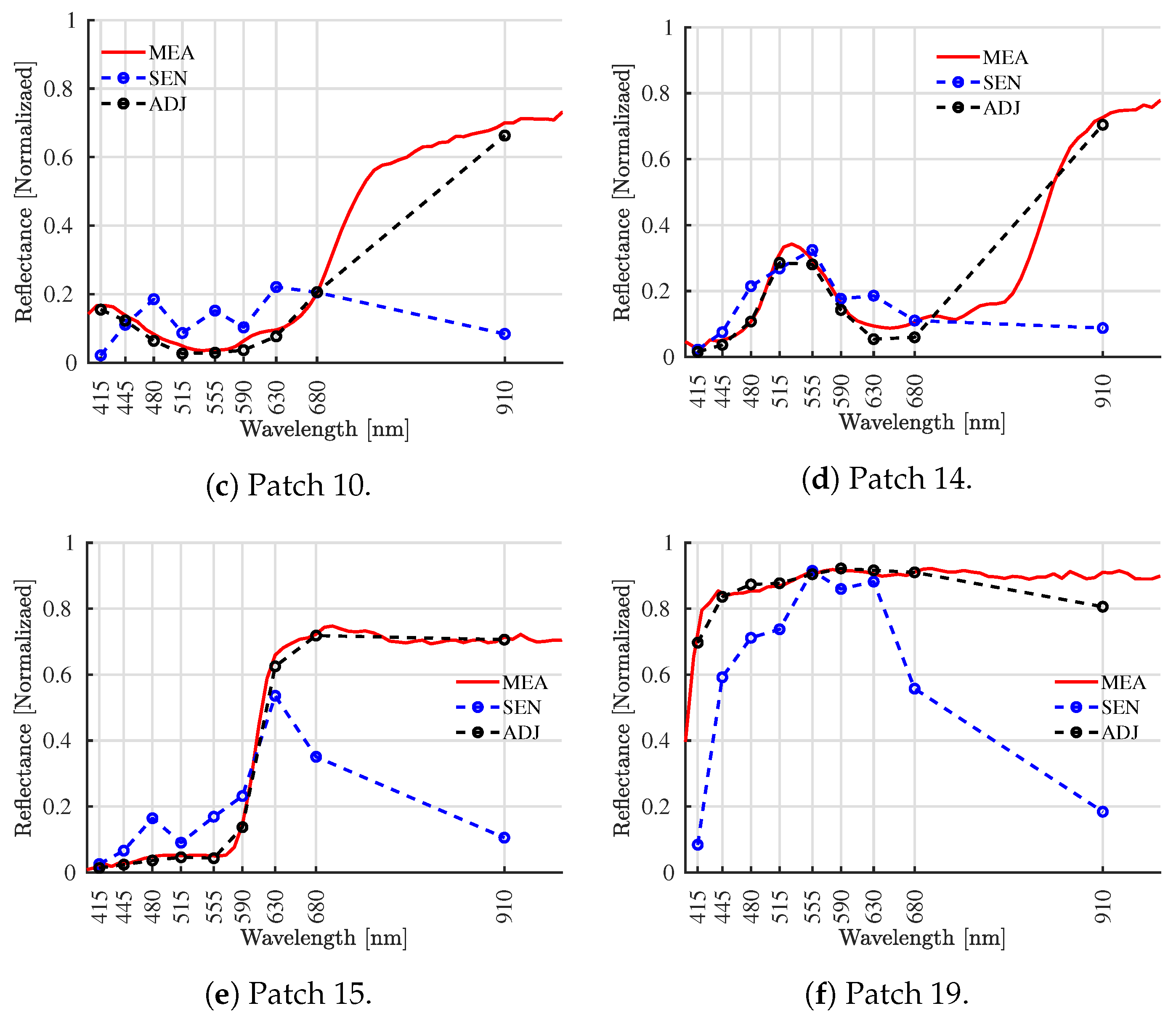
A comparison analysis was conducted to assess the performance of the suggested spectrometer and the implemented ML model. In the initial scenario, the measurements were compared by utilizing the color checker specified in [
33] as the reference technique. There, the authors report the reflectance curves of 24 different patches. All these reference patches were then experimentally characterized using the proposed low-cost spectrometer.
Figure 8 shows only six of them for clarity (patch 01, patch 04, patch 10, patch 14, patch 15, and patch 19). A comparison of the reference reflectance (MEA), raw reflectance (SEN), and adjusted reflectance (ADJ) is shown in each scenario. The ideal MLP configuration (64 neurons in each of the two hidden layers) was used to obtain the ADJ findings.
Based on the obtained results, it is evident that there was a strong correlation between the MEA and SEN measurements, particularly at shorter wavelengths. Additionally, there were slight discrepancies observed at longer wavelengths. However, these disparities were rectified when employing the ideal machine learning model, hence significantly improving the accuracy of the obtained results. In fact, the methodology utilized successfully achieved a strong correlation between the ADJ results and the reference reflectance values across the whole research range (400 to 980 nm).
On the other hand, a quantitative study of the training error was conducted on the 24 instances. The findings are succinctly presented in
Table 2. This table displays the training error analysis, where SEN represents the absolute error against the raw measurement and ADJ denotes the error with respect to the adjusted values. To conduct a thorough investigation, the MAE analysis was computed for each patch and each channel. The obtained results corroborate that the error was significantly reduced in all cases, even at a wavelength of 910 nm, which was the channel that first exhibited the highest level of inaccuracy. Finally, the overall MAE was calculated. The implemented MLP successfully reduced the obtained overall MAE from 0.2979 to 0.0398. In other words, the proposed model reduced the training error by a factor of at least three.
3.3. Validation Error
A second test was carried out to validate the proposed device. For this particular instance, a total of nine colored paper sheets, each of a distinct color, were examined. The reference method employed was the setup outlined in
Section 2.6, wherein measurements were conducted with the Yokogawa AQ6373 optical spectrum analyzer, which is a sophisticated instrument known for its high resolution.
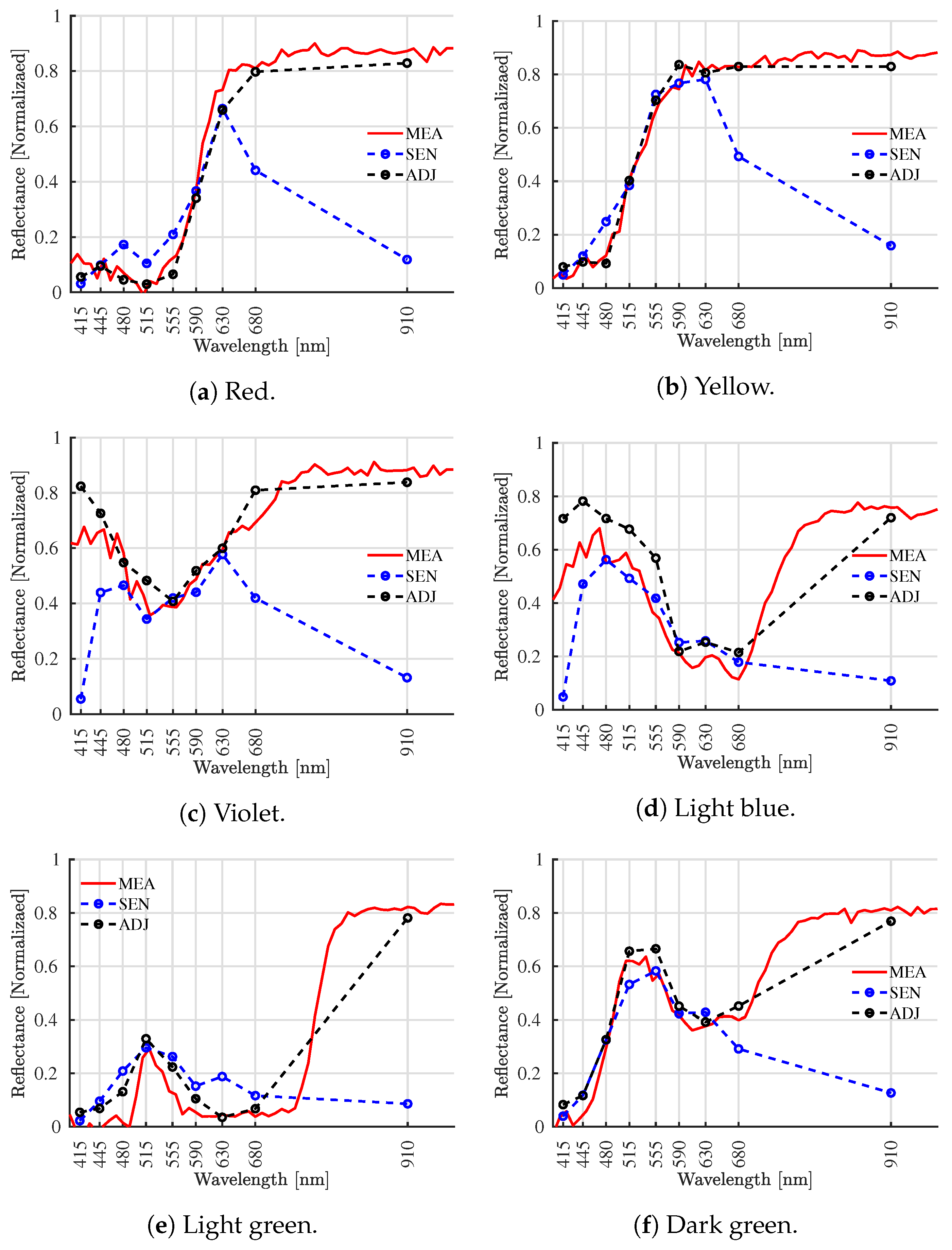
Figure 9 demonstrates the outcomes achieved by utilizing only six out of the nine colored paper sheets, specifically the red, yellow, light-blue, light-green, violet, and dark-green sheets. As in the previous case study, MEA refers to the reference reflectance obtained with the OSA. The raw reflectance is denoted as SEN, and ADJ represents the adjusted reflectance obtained using the best MLP setup.
As in the prior case, the spectrometer provided the correct results, especially at shorter wavelengths. Furthermore, the proposed correction model greatly improved the findings by lowering the difference between the reference reflectance and the obtained reflectance. The results show that the MLP-based model was well-suited for these circumstances, as it allowed for adjustments even when dealing with highly nonlinear reflectance behavior, which is fundamentally complex. For example, while evaluating the red paper sheet (see
Figure 9a), reflectance values of more than 0.8 were found for wavelengths greater than 630 nm. Similarly, when inspecting the violet paper sheet, there was a fall in reflectance between 445 nm and 630 nm (see
Figure 9c), indicating substantial absorption within this range, which is consistent with prior studies.
Table 3 shows the detailed error for each band and each color analyzed with the OSA. Once again, SEN refers to the raw sensor data, and ADJ refers to the data adjusted with the selected MLP. It can be observed that the MAE in this case decreased from 0.1137 to 0.03901 and that the error after adjustment remained close to that of validation, indicating that there was no significant overfitting during the training. Again, it can be observed that the error before adjustment (SEN) was higher in the 910 nm band, but afterward, the error significantly decreased, and the highest error in the adjusted values (ADJ) was observed in the 415 nm band. It can also be seen that the highest error of the adjusted data was found in C07, corresponding to light blue, with an MAE value of 0.0829.
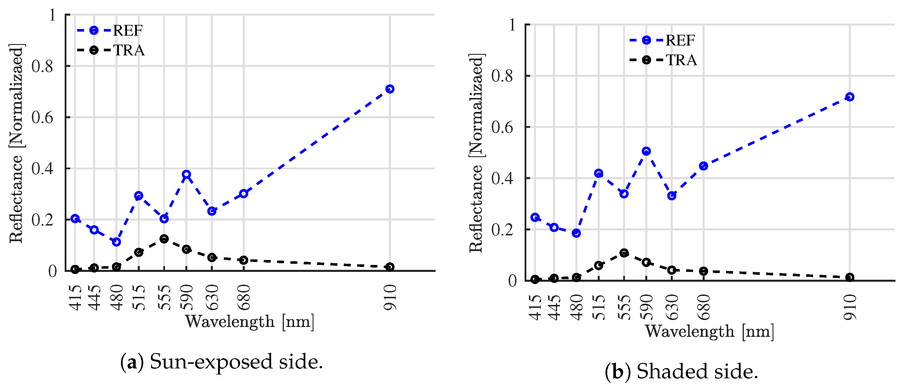
Finally, the proposed spectrometer was employed to analyze and evaluate the optical properties of a plant leaf. Through this practical application, we were able to verify the efficiency of the system in real-life situations, showcasing its value in the spectral analysis of plants, encompassing both reflectance and transmittance.
Figure 10a displays the measured transmittance (TRA) and reflectance (REF) of the sun-exposed side of a leaf, while
Figure 10b illustrates the same parameters for the shaded side of the leaf, as obtained using the suggested affordable spectrometer. As expected, the reflectance of the sun-exposed side was reduced compared with the shaded side of the leaf. This reduction was attributable to the leaf’s optimization for absorbing sunlight efficiently, thereby enhancing its photosynthetic activity. In addition, the drop in the reflectance spectrum curve at 555 nm of a leaf could be attributed to the absorption characteristics of chlorophyll. Chlorophyll, which is the pigment responsible for photosynthesis in plants, absorbs light most efficiently in the blue (427–476 nm) and red (618–780 nm) regions of the electromagnetic spectrum, with minimal absorption in the green region. This phenomenon is known as the “green gap” or “chlorophyll absorption dip”. On the other hand, a considerable increase in reflectance in the infrared band was also expected since plant leaves absorb infrared radiation less efficiently. Infrared radiation is related to heat, and an increase in the reflectance in this region aids in preventing the leaf from overheating.
4. Conclusions
First, a cost-effective and user-friendly optical spectrometer was designed, fabricated, and experimentally validated. This spectrometer employs a training technique based on a comparison with a color checker, which greatly enhances its accuracy and applicability. The training results demonstrated that the machine learning model utilizing a MLP model effectively decreased the training error, even when working with a limited amount of data. Furthermore, the efficacy of the suggested spectrometer in precisely assessing the spectrum of materials exhibiting different colors in the visible and NIR regions was verified by a comparative technique utilizing a high-resolution optical spectrum analyzer. The validation findings indicate that the proposed spectrometer accurately characterized the spectrum properties, and the MAE could be minimized using ML models.
In addition, the integration of a tiny machine learning model within the MCU allowed for real-time data processing and reduced power consumption, enhancing the efficiency and usability of the device. This innovation opens up possibilities for further developments in the field of portable spectroscopy. On the other hand, the proposed device’s capabilities enabled its use in leaf characterization, showcasing its proficiency in analyzing the spectral attributes of leaves in both reflection and transmission. This is particularly advantageous, as certain plants have distinct characteristics or colors on each side of their leaves.
Finally, our research demonstrated the feasibility of creating an optical spectrometer that is not only cost-effective and precise but also user-friendly, with the flexibility to be tailored for diverse applications. The novel training and machine learning techniques we introduced, coupled with the incorporation of real-time learning models, present exciting opportunities for further exploration and advancement in this field. This innovation represents a valuable asset that can be seamlessly integrated into agricultural practices, particularly for the ongoing monitoring of plant health.
Author Contributions
Conceptualization, J.B.-V. and E.R.-V.; software, J.B.-V. and E.O.-R.; visualization, J.B.-V., E.R.-V. and E.O.-R.; methodology, J.B.-V. and E.R.-V.; validation, E.R.-V. and E.O.-R.; original draft preparation, J.B.-V., E.R.-V., E.O.-R. and F.P.-O.; writing—review and editing, J.B.-V., E.R.-V., E.O.-R. and F.P.-O.; funding acquisition, J.B.-V., E.R.-V., E.O.-R. and F.P.-O. All authors read and agreed to the published version of the manuscript.
Funding
This study was suported by the research project “Diseño, desarrollo y validación de un modelo de detección temprana de Tizón Tardío en cultivos de papa Diacol Capiro mediante análisis de imágenes espectrales adquiridas en los departamentos de Boyacá y Cundinamarca”, with the code RC1013-2021 and belonging to the “890-2020 Convocatoria para el fortalecimiento de CTeI en instituciones de educación superior públicas—MINCIENCIAS”.
Informed Consent Statement
Not applicable.
Data Availability Statement
The data presented in this study are available upon request from the corresponding author.
Acknowledgments
This study was supported by the Sistemas de Control y Robótica (GSCR) Research Group COL0123701 at the Sistemas de Control y Robótica Laboratory, which is attached to the Instituto Tecnológico Metropolitano.
Conflicts of Interest
The authors declare no conflicts of interest. The funders had no role in the study’s design; in the collection, analyses, or interpretation of data; in the writing of the manuscript; or in the decision to publish the results.
Abbreviations
The following abbreviations are used in this manuscript:
| LED | Light-emitting diode |
| MLP | Multilayer perceptron |
| MCU | Microcontroller unit |
| VIS-NIR-SWIR | Visible–short-wave near-infrared |
| LWC | Leaf water content |
| SLA | Specific leaf area |
| CHL | Chlorophyll content |
| PLSR | Partial least-squares regression |
| SVR | Support vector regression |
| ML | Machine learning |
| ANN | Artificial neural network |
| IoT | Internet of things |
| NIR | Near-infrared |
| CMOS | Complementary metal-oxide semiconductor |
| BW | Bandwidths |
| ReLU | Rectified linear unit |
| OSA | Optical spectrum analyzer |
| PLA | Polylactic acid |
| ASA | Acrylonitrile styrene acrylate |
| UV | Ultraviolet |
| MAE | Mean absolute error |
| MEA | Reference reflectance |
| SEN | Raw reflectance |
| ADJ | Adjusted reflectance |
References
- Srivastava, S.; Vani, B.; Sadistap, S. Handheld, smartphone based spectrometer for rapid and nondestructive testing of citrus cultivars. J. Food Meas. Charact. 2021, 15, 892–904. [Google Scholar] [CrossRef]
- Li, A.; Yao, C.; ** a soil spectral library using a low-cost NIR spectrometer for precision fertilization in Indonesia. Geoderma Reg. 2020, 22, e00319. [Google Scholar] [CrossRef]
- Ariando, D.; Chen, C.; Greer, M.; Mandal, S. An autonomous, highly portable NMR spectrometer based on a low-cost System-on-Chip (SoC). J. Magn. Reson. 2019, 299, 74–92. [Google Scholar] [CrossRef] [PubMed]
- Kulakowski, J.; d’Humières, B. Chip-size spectrometers drive spectroscopy towards consumer and medical applications. In Proceedings of the Photonic Instrumentation Engineering VIII, Online Only, 6–12 March 2021; Soskind, Y., Busse, L.E., Eds.; SPIE: Bellingham, WA, USA, 2021; p. 44. [Google Scholar] [CrossRef]
- Kim, B.; Jeon, M.; Kim, Y.J.; Choi, S. Open-source, handheld, wireless spectrometer for rapid biochemical assays. Sens. Actuators B Chem. 2020, 306, 127537. [Google Scholar] [CrossRef]
- Gouin-Ferland, B.; Coffee, R.; Therrien, A.C. Data reduction through optimized scalar quantization for more compact neural networks. Front. Phys. 2022, 10, 957128. [Google Scholar] [CrossRef]
- Alajlan, N.N.; Ibrahim, D.M. TinyML: Enabling of Inference Deep Learning Models on Ultra-Low-Power IoT Edge Devices for AI Applications. Micromachines 2022, 13, 851. [Google Scholar] [CrossRef] [PubMed]
- Srinivasagan, R.; Mohammed, M.; Alzahrani, A. TinyML-Sensor for Shelf Life Estimation of Fresh Date Fruits. Sensors 2023, 23, 7081. [Google Scholar] [CrossRef]
- Adafruit. Available online: https://www.adafruit.com/ (accessed on 10 October 2023).
- Monno, Y.; Teranaka, H.; Yoshizaki, K.; Tanaka, M.; Okutomi, M. Single-Sensor RGB-NIR Imaging: High-Quality System Design and Prototype Implementation. IEEE Sens. J. 2019, 19, 497–507. [Google Scholar] [CrossRef]
- Li, K.; Dai, Q.; Xu, W. High quality color calibration for multi-camera systems with an omnidirectional color checker. In Proceedings of the 2010 IEEE International Conference on Acoustics, Speech and Signal Processing, Dallas, TX, USA, 14–19 March 2010; pp. 1026–1029. [Google Scholar] [CrossRef]
- Gendre, L.; Foulonneau, A.; Lapray, P.J.; Bigué, L. Database of polarimetric and multispectral images in the visible and NIR regions. In Proceedings of the Unconventional Optical Imaging, Strasbourg, France, 22–26 April 2018; Fournier, C., Georges, M.P., Popescu, G., Eds.; SPIE: Bellingham, WA, USA, 2018; p. 120. [Google Scholar] [CrossRef]
- Manuel, J.; del Rosario Martinez-Blanco, M.; Viramontes, J.M.C.; Rene, H. Robust Design of Artificial Neural Networks Methodology in Neutron Spectrometry. In Artificial Neural Networks; Suzuki, K., Ed.; IntechOpen: Rijeka, Croatia, 2013; Chapter 4. [Google Scholar] [CrossRef]
- Botero-Valencia, J.S.; Valencia-Aguirre, J.; Durmus, D.; Davis, W. Multi-channel low-cost light spectrum measurement using a multilayer perceptron. Energy Build. 2019, 199, 579–587. [Google Scholar] [CrossRef]
- Jadidi, A.; Mi, Y.; Sikström, F.; Nilsen, M.; Ancona, A. Beam Offset Detection in Laser Stake Welding of Tee Joints Using Machine Learning and Spectrometer Measurements. Sensors 2022, 22, 3881. [Google Scholar] [CrossRef] [PubMed]
- Behkami, S.; Zain, S.M.; Gholami, M.; Khir, M.F.A. Classification of cow milk using artificial neural network developed from the spectral data of single- and three-detector spectrophotometers. Food Chem. 2019, 294, 309–315. [Google Scholar] [CrossRef] [PubMed]
| Disclaimer/Publisher’s Note: The statements, opinions and data contained in all publications are solely those of the individual author(s) and contributor(s) and not of MDPI and/or the editor(s). MDPI and/or the editor(s) disclaim responsibility for any injury to people or property resulting from any ideas, methods, instructions or products referred to in the content. |
© 2024 by the authors. Licensee MDPI, Basel, Switzerland. This article is an open access article distributed under the terms and conditions of the Creative Commons Attribution (CC BY) license (https://creativecommons.org/licenses/by/4.0/).


