
Thawing Permafrost as a Nitrogen Fertiliser: Implications for Climate Feedbacks


Abstract
:1. Introduction
2. Materials and Methods
2.1. JULES Land Surface Scheme
2.2. IMOGEN
2.3. Experimental Design
3. Results and Discussion
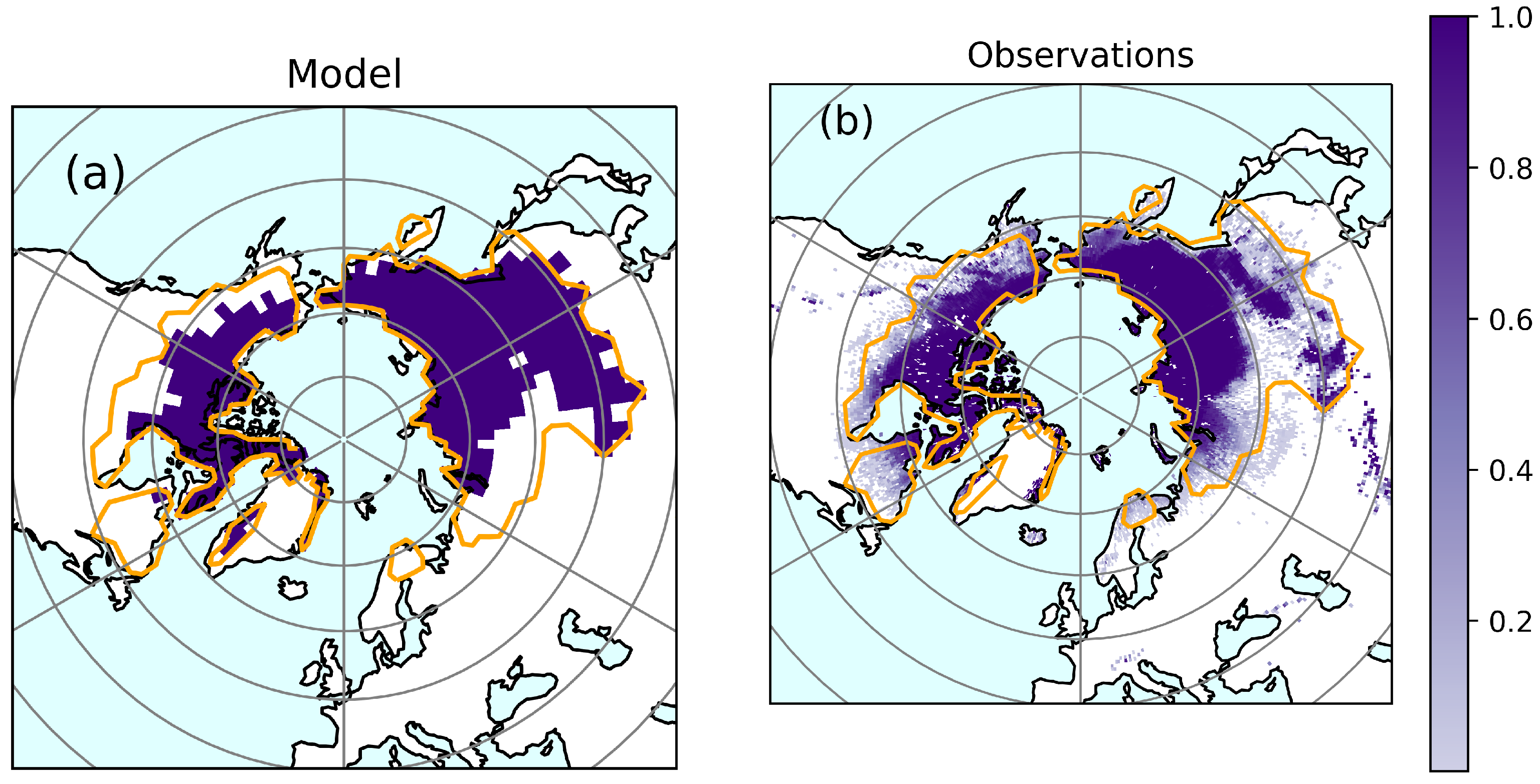
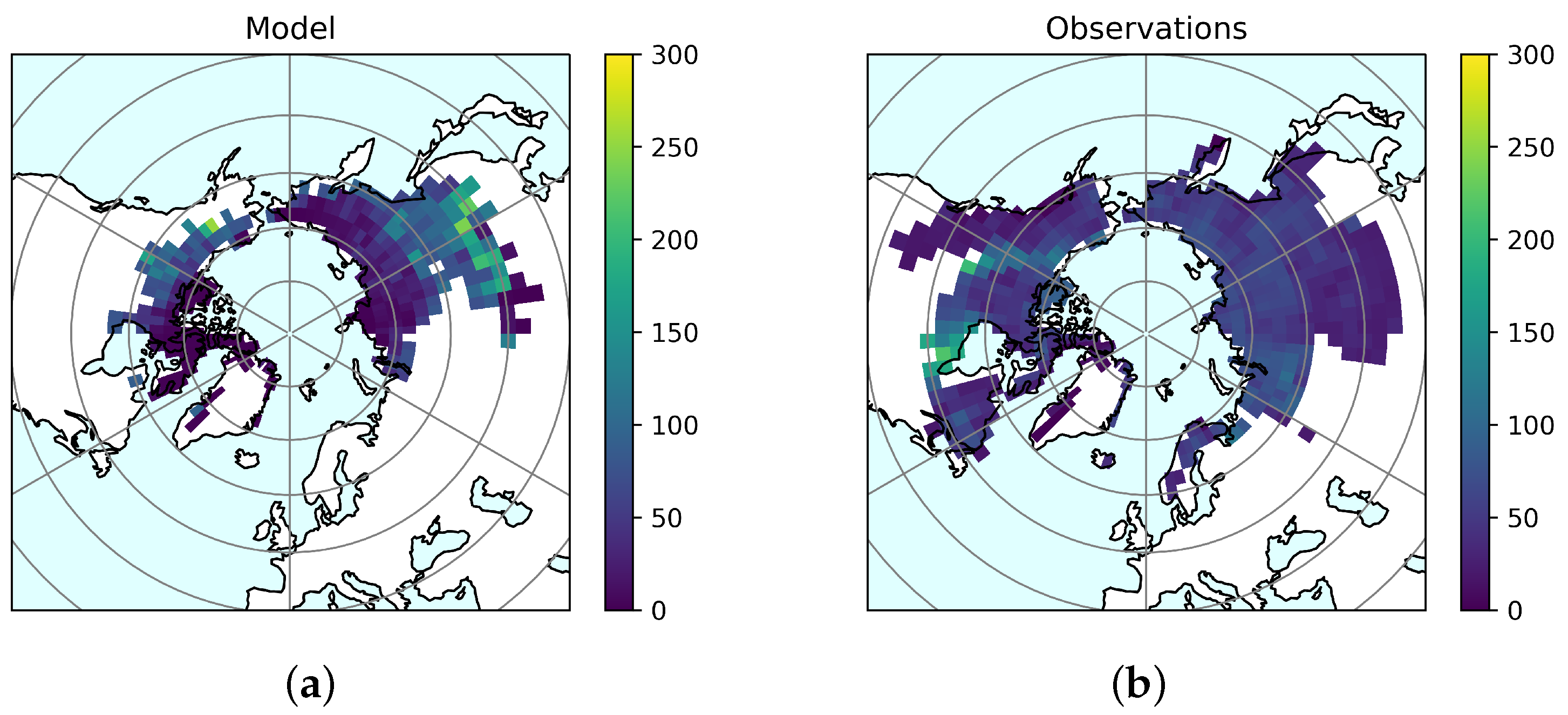
3.1. Model Evaluation
Permafrost Soils
3.2. Projections over the Permafrost Region
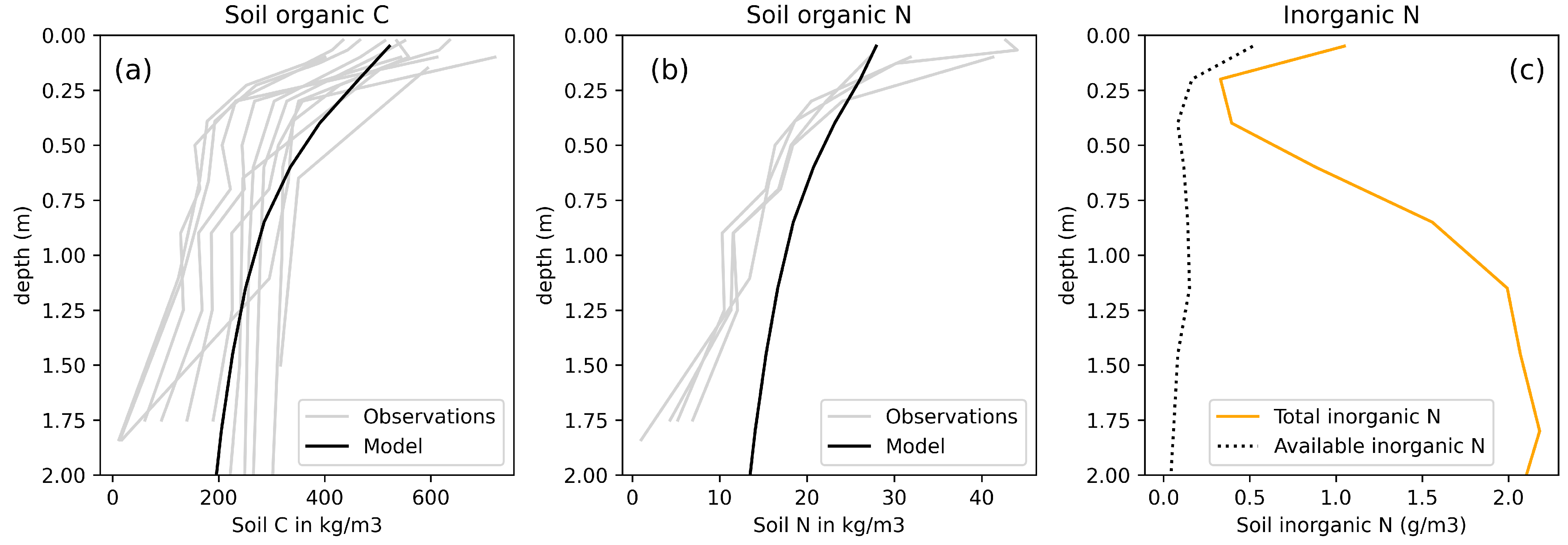
3.2.1. Soil Nitrogen
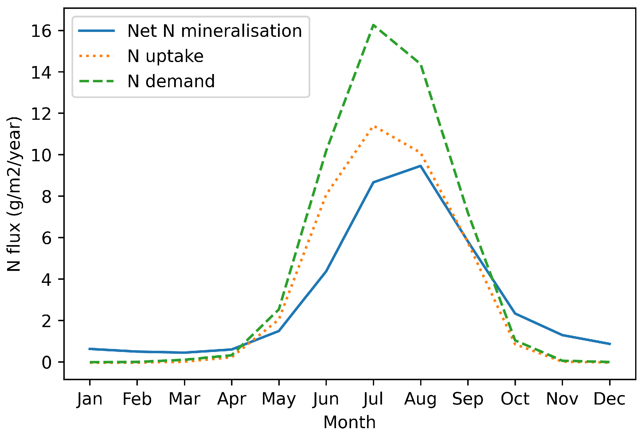
3.2.2. Nitrogen Limitation
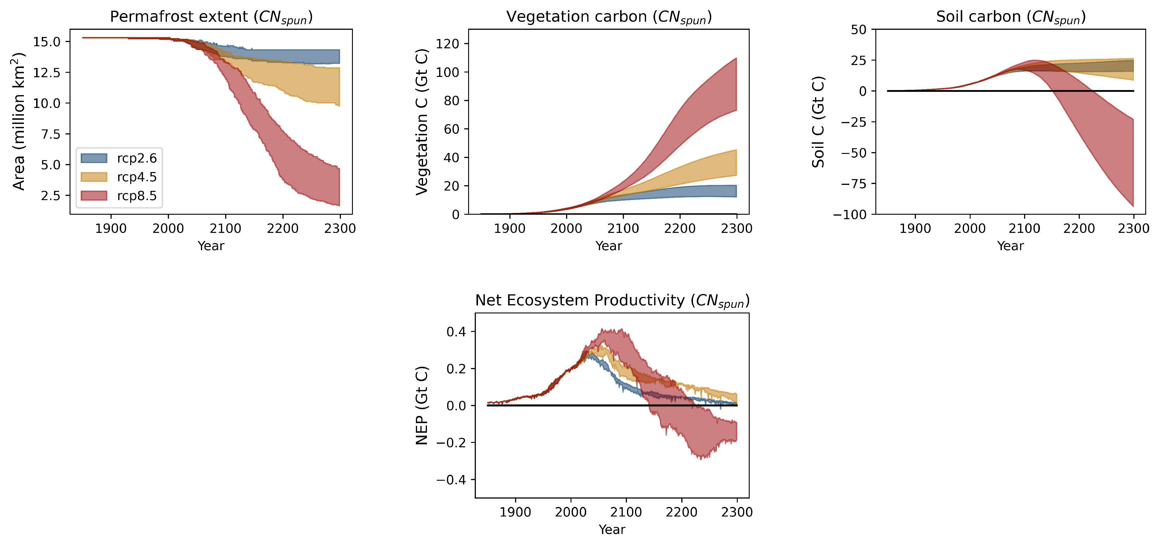
3.2.3. Implications for the Carbon Cycle
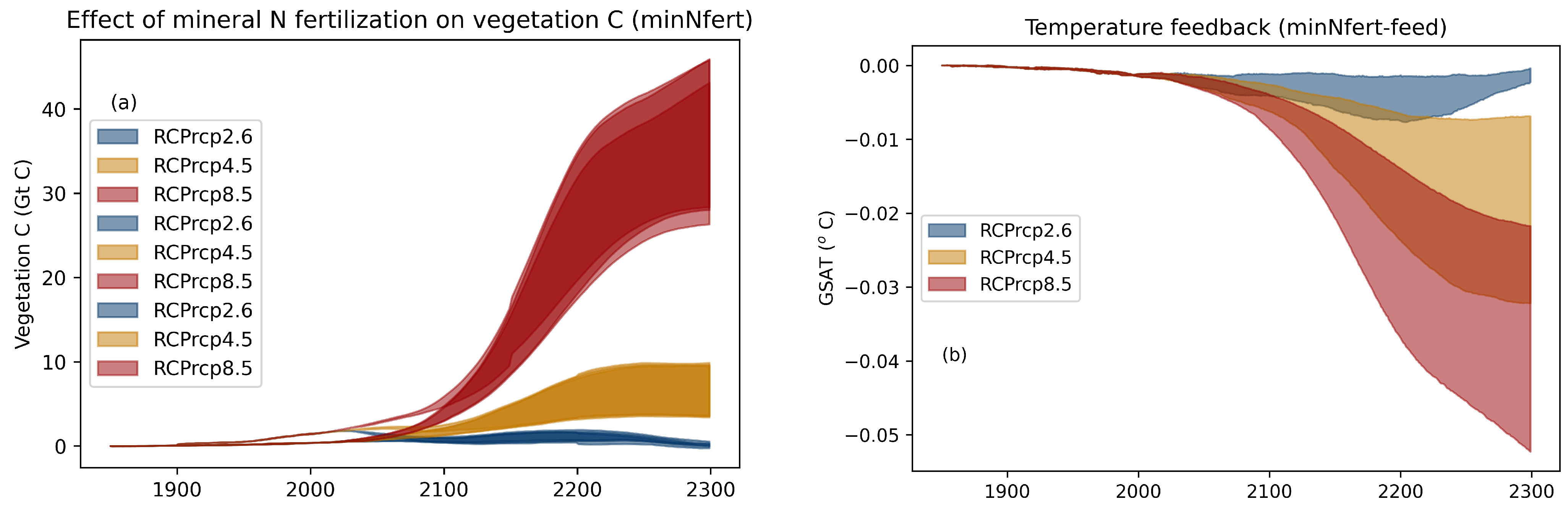
3.3. Mineral Nitrogen Vegetation Fertilisation (minNfert) and Feedback (minNfert-Feed)
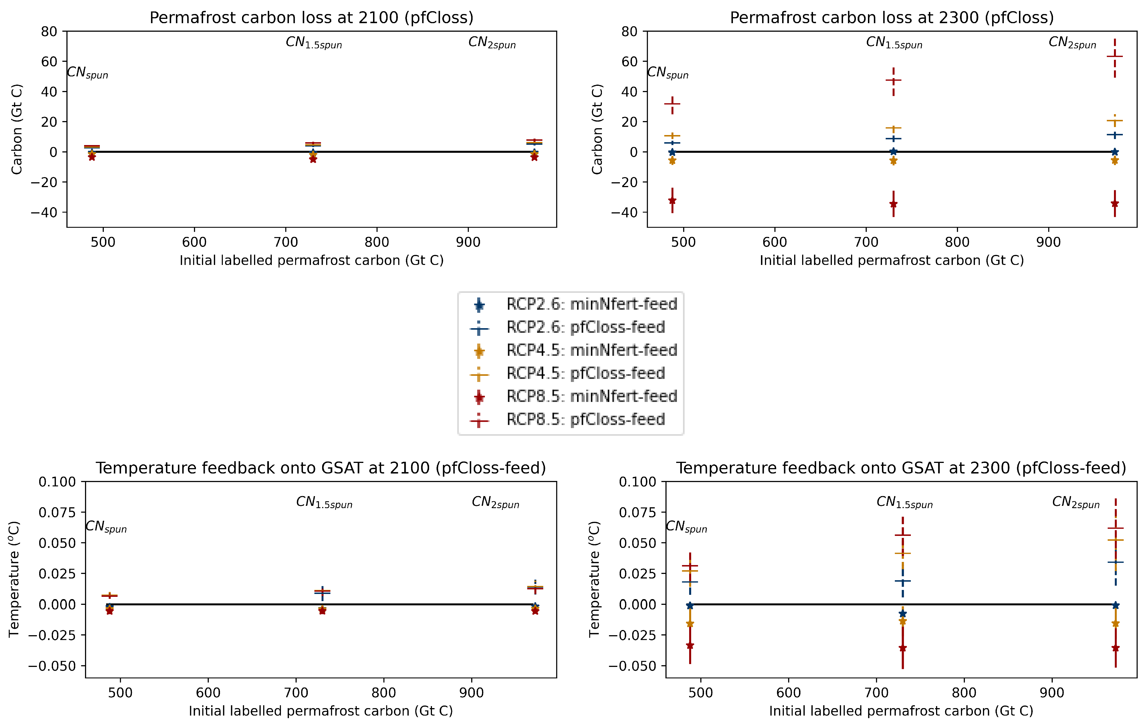
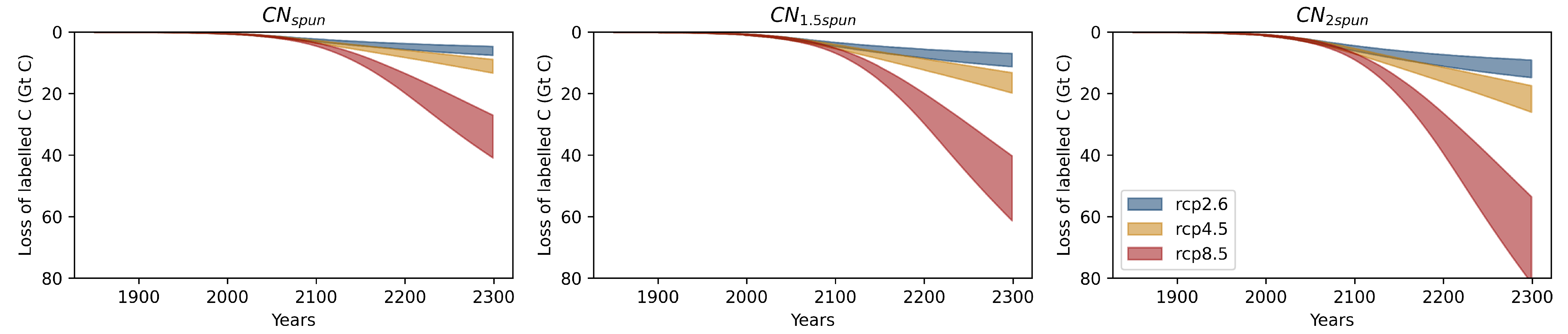
3.4. Comparison with the Permafrost Carbon Feedback (pfCloss-Feed)
4. Discussion and Conclusions
Supplementary Materials
Author Contributions
Funding
Institutional Review Board Statement
Informed Consent Statement
Data Availability Statement
Conflicts of Interest
Appendix A. The Permafrost Carbon Feedback
Appendix A.1. Revised Methodology for Estimating the Permafrost Carbon Feedback Temperature


Appendix A.2. Impact of the Initial Conditions the Permafrost Carbon Feedback Temperature


References
- Obu, J.; Westermann, S.; Bartsch, A.; Berdnikov, N.; Christiansen, H.H.; Dashtseren, A.; Delaloye, R.; Elberling, B.; Etzelmüller, B.; Kholodov, A.; et al. Northern Hemisphere permafrost map based on TTOP modelling for 2000–2016 at 1 km2 scale. Earth-Sci. Rev. 2019, 193, 299–316. [Google Scholar] [CrossRef]
- Zhang, T.; Heginbottom, J.A.; Barry, R.G.; Brown, J. Further statistics on the distribution of permafrost and ground ice in the Northern Hemisphere. Polar Geogr. 2000, 24, 126–131. [Google Scholar] [CrossRef]
- Biskaborn, B.; Smith, S.; Noetzli, J.; Matthes, H.; Vieira, G.; Streletskiy, D.; Schoeneich, P.; Romanovsky, V.; Lewkowicz, A.; Abramov, A.; et al. Permafrost is warming at a global scale. Nat. Commun. 2019, 10, 264. [Google Scholar] [CrossRef] [PubMed] [Green Version]
- Pörtner, H.O.; Roberts, D.; Masson-Delmotte, V.; Zhai, P.; Tignor, M.; Poloczanska, E.; Mintenbeck, K.; Nicolai, M.; Okem, A.; Petzold, J.; et al. IPCC, 2019: Summary for Policymaker. In Special Report on the Ocean and Cryosphere in a Changing Climate; IPCC: Geneva, Switzerland, 2019. [Google Scholar]
- Chadburn, S.E.; Burke, E.; Cox, P.; Friedlingstein, P.; Hugelius, G.; Westermann, S. An observation-based constraint on permafrost loss as a function of global warming. Nat. Clim. Chang. 2017, 7, 340–344. [Google Scholar] [CrossRef]
- Burke, E.J.; Ekici, A.; Huang, Y.; Chadburn, S.E.; Huntingford, C.; Ciais, P.; Friedlingstein, P.; Peng, S.; Krinner, G. Quantifying uncertainties of permafrost carbon–climate feedbacks. Biogeosciences 2017, 14, 3051–3066. [Google Scholar] [CrossRef] [Green Version]
- Vonk, J.E.; Tank, S.E.; Bowden, W.B.; Laurion, I.; Vincent, W.F.; Alekseychik, P.; Amyot, M.; Billet, M.; Canario, J.; Cory, R.M.; et al. Reviews and syntheses: Effects of permafrost thaw on Arctic aquatic ecosystems. Biogeosciences 2015, 12, 7129–7167. [Google Scholar] [CrossRef] [Green Version]
- Wotton, B.; Flannigan, M.; Marshall, G. Potential climate change impacts on fire intensity and key wildfire suppression thresholds in Canada. Environ. Res. Lett. 2017, 12, 095003. [Google Scholar] [CrossRef]
- Melvin, A.M.; Larsen, P.; Boehlert, B.; Neumann, J.E.; Chinowsky, P.; Espinet, X.; Martinich, J.; Baumann, M.S.; Rennels, L.; Alexandra, B.; et al. Climate change damages to Alaska public infrastructure and the economics of proactive adaptation. Proc. Natl. Acad. Sci. USA 2017, 114, E122–E131. [Google Scholar] [CrossRef] [Green Version]
- Hjort, J.; Karjalainen, O.; Aalto, J.; Westermann, S.; Romanovsky, V.E.; Nelson, F.E.; Etzelmüller, B.; Luoto, M. Degrading permafrost puts Arctic infrastructure at risk by mid-century. Nat. Commun. 2018, 9, 5147. [Google Scholar] [CrossRef]
- Larsen, J.; Anisimov, O.; Constable, A.; Hollowed, A.; Maynard, N.; Prestrud, P.; Prowse, T.; Stone, J. Climate Change 2014: Impacts, Adaptation, and Vulnerability Part B: Regional Aspects; Contribution of Working Group II to the Fifth Assessment Report of the Intergovernmental Panel of Climate Change; Barros, V.R., Field, C.B., Dokken, D.J., Mastrandrea, M.D., Mach, K.J., Bilir, T.E., Chatterjee, M., Ebi, K.L., Estrada, Y.O., Genova, R.C., et al., Eds.; Cambridge University Press: Cambridge, UK, 2014. [Google Scholar]
- Turetsky, M.R.; Abbott, B.W.; Jones, M.C.; Anthony, K.W.; Olefeldt, D.; Schuur, E.A.; Grosse, G.; Kuhry, P.; Hugelius, G.; Koven, C.; et al. Carbon release through abrupt permafrost thaw. Nat. Geosci. 2020, 13, 138–143. [Google Scholar] [CrossRef]
- Schuur, E.A.; McGuire, A.D.; Schädel, C.; Grosse, G.; Harden, J.; Hayes, D.J.; Hugelius, G.; Koven, C.D.; Kuhry, P.; Lawrence, D.M.; et al. Climate change and the permafrost carbon feedback. Nature 2015, 520, 171–179. [Google Scholar] [CrossRef]
- Wiltshire, A.J.; Burke, E.J.; Chadburn, S.E.; Jones, C.D.; Cox, P.M.; Davies-Barnard, T.; Friedlingstein, P.; Harper, A.B.; Liddicoat, S.; Sitch, S.; et al. JULES-CN: A coupled terrestrial carbon–nitrogen scheme (JULES vn5.1). Geosci. Model Dev. 2021, 14, 2161–2186. [Google Scholar] [CrossRef]
- Chapin, F.S., III; Shaver, G.R.; Giblin, A.E.; Nadelhoffer, K.J.; Laundre, J.A. Responses of arctic tundra to experimental and observed changes in climate. Ecology 1995, 76, 694–711. [Google Scholar] [CrossRef]
- Finger, R.A.; Turetsky, M.R.; Kielland, K.; Ruess, R.W.; Mack, M.C.; Euskirchen, E.S. Effects of permafrost thaw on nitrogen availability and plant–soil interactions in a boreal Alaskan lowland. J. Ecol. 2016, 104, 1542–1554. [Google Scholar] [CrossRef]
- Keuper, F.; Dorrepaal, E.; van Bodegom, P.M.; van Logtestijn, R.; Venhuizen, G.; van Hal, J.; Aerts, R. Experimentally increased nutrient availability at the permafrost thaw front selectively enhances biomass production of deep-rooting subarctic peatland species. Glob. Chang. Biol. 2017, 23, 4257–4266. [Google Scholar] [CrossRef]
- Salmon, V.G.; Soucy, P.; Mauritz, M.; Celis, G.; Natali, S.M.; Mack, M.C.; Schuur, E.A. Nitrogen availability increases in a tundra ecosystem during five years of experimental permafrost thaw. Glob. Chang. Biol. 2016, 22, 1927–1941. [Google Scholar] [CrossRef] [PubMed]
- Beermann, F.; Langer, M.; Wetterich, S.; Strauss, J.; Boike, J.; Fiencke, C.; Schirrmeister, L.; Pfeiffer, E.M.; Kutzbach, L. Permafrost Thaw and Liberation of Inorganic Nitrogen in Eastern Siberia. Permafr. Periglac. Process. 2017, 28, 605–618. [Google Scholar] [CrossRef] [Green Version]
- Harden, J.W.; Koven, C.D.; **, C.L.; Hugelius, G.; McGuire, A.D.; Camill, P.; Jorgenson, T.; Kuhry, P.; Michaelson, G.J.; O’Donnell, J.A.; et al. Field information links permafrost carbon to physical vulnerabilities of thawing. Geophys. Res. Lett. 2012, 39, L15704. [Google Scholar] [CrossRef] [Green Version]
- Wang, P.; Limpens, J.; Mommer, L.; van Ruijven, J.; Nauta, A.L.; Berendse, F.; Schaepman-Strub, G.; Blok, D.; Maximov, T.C.; Heijmans, M.M. Above-and below-ground responses of four tundra plant functional types to deep soil heating and surface soil fertilization. J. Ecol. 2017, 105, 947–957. [Google Scholar] [CrossRef] [Green Version]
- Hewitt, R.E.; Taylor, D.L.; Genet, H.; McGuire, A.D.; Mack, M.C. Below-ground plant traits influence tundra plant acquisition of newly thawed permafrost nitrogen. J. Ecol. 2019, 107, 950–962. [Google Scholar] [CrossRef]
- Koven, C.D.; Lawrence, D.M.; Riley, W.J. Permafrost carbon-climate feedback is sensitive to deep soil carbon decomposability but not deep soil nitrogen dynamics. Proc. Natl. Acad. Sci. USA 2015, 112, 3752–3757. [Google Scholar] [CrossRef] [PubMed] [Green Version]
- Keuper, F.; Bodegom, P.M.; Dorrepaal, E.; Weedon, J.T.; Hal, J.; Logtestijn, R.S.; Aerts, R. A frozen feast: Thawing permafrost increases plant-available nitrogen in subarctic peatlands. Glob. Chang. Biol. 2012, 18, 1998–2007. [Google Scholar] [CrossRef]
- Sellar, A.A.; Jones, C.G.; Mulcahy, J.; Tang, Y.; Yool, A.; Wiltshire, A.; O’connor, F.M.; Stringer, M.; Hill, R.; Palmieri, J.; et al. UKESM1: Description and evaluation of the UK Earth System Model. J. Adv. Model. Earth Syst. 2019, 11, 4513–4558. [Google Scholar] [CrossRef] [Green Version]
- Best, M.; Pryor, M.; Clark, D.; Rooney, G.; Essery, R.; Ménard, C.; Edwards, J.; Hendry, M.; Porson, A.; Gedney, N.; et al. The Joint UK Land Environment Simulator (JULES), model description–Part 1: Energy and water fluxes. Geosci. Model Dev. 2011, 4, 677–699. [Google Scholar] [CrossRef] [Green Version]
- Clark, D.; Mercado, L.; Sitch, S.; Jones, C.; Gedney, N.; Best, M.; Pryor, M.; Rooney, G.; Essery, R.; Blyth, E.; et al. The Joint UK Land Environment Simulator (JULES), model description–Part 2: Carbon fluxes and vegetation dynamics. Geosci. Model Dev. 2011, 4, 701–722. [Google Scholar] [CrossRef] [Green Version]
- Harper, A.B.; Cox, P.M.; Friedlingstein, P.; Wiltshire, A.J.; Jones, C.D.; Sitch, S.; Mercado, L.M.; Groenendijk, M.; Robertson, E.; Kattge, K.; et al. Improved representation of plant functional types and physiology in the Joint UK Land Environment Simulator (JULES v4.2) using plant trait information. Geosci. Model Dev. 2016, 9, 2415–2440. [Google Scholar] [CrossRef] [Green Version]
- Burke, E.J.; Chadburn, S.E.; Ekici, A. A vertical representation of soil carbon in the JULES land surface scheme (vn4.3_permafrost) with a focus on permafrost regions. Geosci. Model Dev. 2017, 10, 959–975. [Google Scholar] [CrossRef] [Green Version]
- Burke, E.J.; Chadburn, S.E.; Huntingford, C.; Jones, C.D. CO2 loss by permafrost thawing implies additional emissions reductions to limit warming to 1.5 or 2 °C. Environ. Res. Lett. 2018, 13, 024024. [Google Scholar] [CrossRef]
- Huntingford, C.; Booth, B.; Sitch, S.; Gedney, N.; Lowe, J.; Liddicoat, S.; Mercado, L.; Best, M.; Weedon, G.; Fisher, R.; et al. IMOGEN: An intermediate complexity model to evaluate terrestrial impacts of a changing climate. Geosci. Model Dev. 2010, 3, 679–687. [Google Scholar] [CrossRef] [Green Version]
- Huntingford, C.; Cox, P. An analogue model to derive additional climate change scenarios from existing GCM simulations. Clim. Dyn. 2000, 16, 575–586. [Google Scholar] [CrossRef]
- Comyn-Platt, E.; Hayman, G.; Huntingford, C.; Chadburn, S.E.; Burke, E.J.; Harper, A.B.; Collins, W.J.; Webber, C.P.; Powell, T.; Cox, P.M.; et al. Carbon budgets for 1.5 and 2 °C targets lowered by natural wetland and permafrost feedbacks. Nat. Geosci. 2018, 11, 568–573. [Google Scholar] [CrossRef]
- Zelazowski, P.; Huntingford, C.; Mercado, L.M.; Schaller, N. Climate pattern-scaling set for an ensemble of 22 GCMs—Adding uncertainty to the IMOGEN version 2.0 impact system. Geosci. Model Dev. 2018, 11, 541–560. [Google Scholar] [CrossRef] [Green Version]
- Weedon, G.; Gomes, S.; Viterbo, P.; Shuttleworth, W.J.; Blyth, E.; Österle, H.; Adam, J.; Bellouin, N.; Boucher, O.; Best, M. Creation of the WATCH forcing data and its use to assess global and regional reference crop evaporation over land during the twentieth century. J. Hydrometeorol. 2011, 12, 823–848. [Google Scholar] [CrossRef] [Green Version]
- Moss, R.H.; Edmonds, J.A.; Hibbard, K.A.; Manning, M.R.; Rose, S.K.; Van Vuuren, D.P.; Carter, T.R.; Emori, S.; Kainuma, M.; Kram, T.; et al. The next generation of scenarios for climate change research and assessment. Nature 2010, 463, 747–756. [Google Scholar] [CrossRef]
- Meinshausen, M.; Smith, S.J.; Calvin, K.; Daniel, J.S.; Kainuma, M.; Lamarque, J.F.; Matsumoto, K.; Montzka, S.; Raper, S.; Riahi, K.; et al. The RCP greenhouse gas concentrations and their extensions from 1765 to 2300. Clim. Change 2011, 109, 213. [Google Scholar] [CrossRef] [Green Version]
- Brown, J.; Hinkel, K.M.; Nelson, F.E. Circumpolar Active Layer Monitoring (CALM) Program Network; National Snow and Ice Data Center: Boulder, CO, USA, 2003. [Google Scholar]
- Weedon, G.P.; Balsamo, G.; Bellouin, N.; Gomes, S.; Best, M.J.; Viterbo, P. The WFDEI meteorological forcing data set: WATCH Forcing Data methodology applied to ERA-Interim reanalysis data. Water Resour. Res. 2014, 50, 7505–7514. [Google Scholar] [CrossRef] [Green Version]
- Harper, A.B.; Wiltshire, A.J.; Cox, P.M.; Friedlingstein, P.; Jones, C.D.; Mercado, L.M.; Sitch, S.; Williams, K.; Duran-Rojas, C. Vegetation distribution and terrestrial carbon cycle in a carbon-cycle configuration of JULES4.6 with new plant functional types. Geosci. Model Dev. 2018, 11, 2857–2873. [Google Scholar] [CrossRef] [Green Version]
- Olson, D.M.; Dinerstein, E.; Wikramanayake, E.D.; Burgess, N.D.; Powell, G.V.; Underwood, E.C.; D’amico, J.A.; Itoua, I.; Strand, H.E.; Morrison, J.C.; et al. Terrestrial Ecoregions of the World: A New Map of Life on Earth A new global map of terrestrial ecoregions provides an innovative tool for conserving biodiversity. BioScience 2001, 51, 933–938. [Google Scholar] [CrossRef]
- Burke, E.J.; Zhang, Y.; Krinner, G. Evaluating permafrost physics in the Coupled Model Intercomparison Project 6 (CMIP6) models and their sensitivity to climate change. Cryosphere 2020, 14, 3155–3174. [Google Scholar] [CrossRef]
- Urban, M.; Hese, S.; Herold, M.; Pöcking, S.; Schmullius, C. Pan-Arctic Land Cover map** and fire assessment for the ESA data user element Permafrost. PFG Photogramm. Fernerkund. Geoinf. 2010, 14, 283–293. [Google Scholar] [CrossRef]
- Ruesch, A.; Gibb, H. New IPCC Tier-1 Global Biomass Carbon Map For the Year 2000. 2000. Available online: https://data.ess-dive.lbl.gov/view/doi:10.15485/1463800 (accessed on 20 March 2022).
- Jung, M.; Reichstein, M.; Margolis, H.A.; Cescatti, A.; Richardson, A.D.; Arain, M.A.; Arneth, A.; Bernhofer, C.; Bonal, D.; Chen, J.; et al. Global patterns of land-atmosphere fluxes of carbon dioxide, latent heat, and sensible heat derived from eddy covariance, satellite, and meteorological observations. J. Geophys. Res. Biogeosci. 2011, 116, G00J07. [Google Scholar] [CrossRef] [Green Version]
- Zhao, M.; Running, S.W. Drought-induced reduction in global terrestrial net primary production from 2000 through 2009. Science 2010, 329, 940–943. [Google Scholar] [CrossRef] [PubMed] [Green Version]
- Bloom, A.A.; Exbrayat, J.F.; Van Der Velde, I.R.; Feng, L.; Williams, M. The decadal state of the terrestrial carbon cycle: Global retrievals of terrestrial carbon allocation, pools, and residence times. Proc. Natl. Acad. Sci. USA 2016, 113, 1285–1290. [Google Scholar] [CrossRef] [PubMed] [Green Version]
- Carvalhais, N.; Forkel, M.; Khomik, M.; Bellarby, J.; Jung, M.; Migliavacca, M.; Mu, M.; Saatchi, S.; Santoro, M.; Thurner, M.; et al. Global covariation of carbon turnover times with climate in terrestrial ecosystems. Nature 2014, 514, 213–217. [Google Scholar] [CrossRef] [PubMed] [Green Version]
- Hugelius, G.; Strauss, J.; Zubrzycki, S.; Harden, J.W.; Schuur, E.; **, C.L.; Schirrmeister, L.; Grosse, G.; Michaelson, G.J.; Koven, C.D.; et al. Estimated stocks of circumpolar permafrost carbon with quantified uncertainty ranges and identified data gaps. Biogeosciences 2014, 11, 6573–6593. [Google Scholar] [CrossRef] [Green Version]
- Schulte-Uebbing, L.; de Vries, W. Global-scale impacts of nitrogen deposition on tree carbon sequestration in tropical, temperate, and boreal forests: A meta-analysis. Glob. Chang. Biol. 2018, 24, e416–e431. [Google Scholar] [CrossRef]
- LeBauer, D.S.; Treseder, K.K. Nitrogen limitation of net primary productivity in terrestrial ecosystems is globally distributed. Ecology 2008, 89, 371–379. [Google Scholar] [CrossRef] [Green Version]
- Global Soil Data Task Group. Global Gridded Surfaces of Selected Soil Characteristics (IGBP-DIS); ORNL DAAC: Oak Ridge, TN, USA, 2000. [Google Scholar] [CrossRef]
- Salmon, V.G.; Schädel, C.; Bracho, R.; Pegoraro, E.; Celis, G.; Mauritz, M.; Mack, M.C.; Schuur, E.A. Adding depth to our understanding of nitrogen dynamics in permafrost soils. J. Geophys. Res. Biogeosci. 2018, 123, 2497–2512. [Google Scholar] [CrossRef]
- Wild, B.; Alves, R.J.E.; Bárta, J.; Čapek, P.; Gentsch, N.; Guggenberger, G.; Hugelius, G.; Knoltsch, A.; Kuhry, P.; Lashchinskiy, N.; et al. Amino acid production exceeds plant nitrogen demand in Siberian tundra. Environ. Res. Lett. 2018, 13, 034002. [Google Scholar] [CrossRef]
- Pedersen, E.P.; Elberling, B.; Michelsen, A. Foraging deeply: Depth-specific plant nitrogen uptake in response to climate-induced N-release and permafrost thaw in the High Arctic. Glob. Chang. Biol. 2020, 26, 6523–6536. [Google Scholar] [CrossRef]
- McGuire, A.D.; Lawrence, D.M.; Koven, C.; Clein, J.S.; Burke, E.; Chen, G.; Jafarov, E.; MacDougall, A.H.; Marchenko, S.; Nicolsky, D.; et al. Dependence of the evolution of carbon dynamics in the northern permafrost region on the trajectory of climate change. Proc. Natl. Acad. Sci. USA 2018, 115, 3882–3887. [Google Scholar] [CrossRef] [PubMed] [Green Version]
- Voigt, C.; Marushchak, M.E.; Abbott, B.W.; Biasi, C.; Elberling, B.; Siciliano, S.D.; Sonnentag, O.; Stewart, K.J.; Yang, Y.; Martikainen, P.J. Nitrous oxide emissions from permafrost-affected soils. Nat. Rev. Earth Environ. 2020, 1, 420–434. [Google Scholar] [CrossRef]
- Witze, A. The Arctic is burning like never before—And that’s bad news for climate change. Nature 2020, 585, 336–337. [Google Scholar] [CrossRef] [PubMed]
- Turetsky, M.R.; Abbott, B.W.; Jones, M.C.; Anthony, K.W.; Olefeldt, D.; Schuur, E.A.; Koven, C.; McGuire, A.D.; Grosse, G.; Kuhry, P.; et al. Permafrost collapse is accelerating carbon release. Nature 2019, 569, 32–34. [Google Scholar] [CrossRef] [Green Version]
- Sanderman, J.; Hengl, T.; Fiske, G.J. Soil carbon debt of 12,000 years of human land use. Proc. Natl. Acad. Sci. USA 2017, 114, 9575–9580. [Google Scholar] [CrossRef] [Green Version]
- Fan, N.; Koirala, S.; Reichstein, M.; Thurner, M.; Avitabile, V.; Santoro, M.; Ahrens, B.; Weber, U.; Carvalhais, N. Apparent ecosystem carbon turnover time: Uncertainties and robust features. Earth Syst. Sci. Data 2020, 12, 2517–2536. [Google Scholar] [CrossRef]
- Batjes, N.H. Harmonized soil property values for broad-scale modelling (WISE30sec) with estimates of global soil carbon stocks. Geoderma 2016, 269, 61–68. [Google Scholar] [CrossRef]
- Batjes, N. Harmonized soil profile data for applications at global and continental scales: Updates to the WISE database. Soil Use Manag. 2009, 25, 124–127. [Google Scholar] [CrossRef]
- Shangguan, W.; Dai, Y.; Duan, Q.; Liu, B.; Yuan, H. A global soil data set for earth system modeling. J. Adv. Model. Earth Syst. 2014, 6, 249–263. [Google Scholar] [CrossRef]
- Parsons, M.; Zhang, T. CAPS: The Circumpolar Active-Layer and Permafrost System, version 2.0; National Snow and Ice Data Center: Boulder, CO, USA, 2003. [Google Scholar]
- Biskaborn, B.K.; Lanckman, J.P.; Lantuit, H.; Elger, K.; Dmitry, S.; William, C.; Vladimir, R. The new database of the Global Terrestrial Network for Permafrost (GTN-P). Earth Syst. Sci. Data 2015, 7, 245–259. [Google Scholar] [CrossRef] [Green Version]


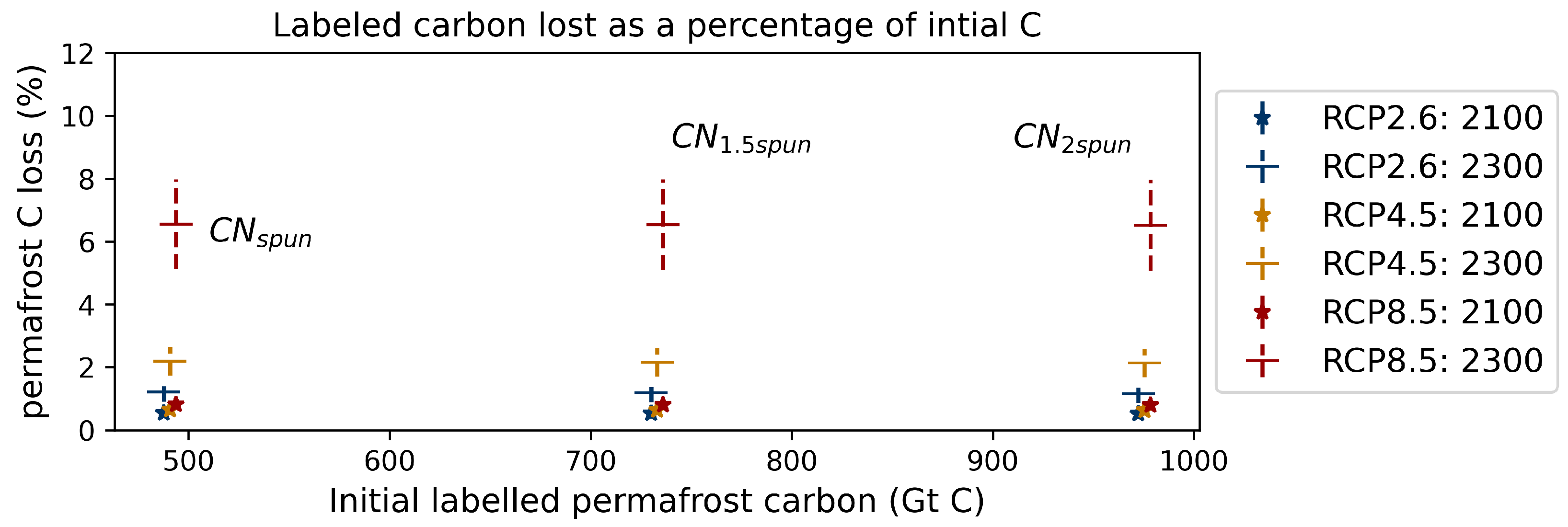
| Simulation Name | Permafrost C Initiation Method | Labelled Permafrost C (Gt C) |
|---|---|---|
| Spun up until stable | 484 | |
| Prescribed (1.5 × ) | 727 | |
| Prescribed (2 × | 969 |
| Ensemble Name | Description |
|---|---|
| transient-ens Main simulations | Transient runs for 3 scenarios (RCP8.5, 4.5 and 2.6) with prescribed CO emissions and N deposition. Each individual ensemble member is compared with the 4 additional diagnostic experiments described below to quantify: • Vegetation fertilisation by mineral N released by thawing permafrost (minNfert) • Temperature feedback of vegetation C response onto global climate (minNfert-feed) • Permafrost carbon loss (pfCloss) • Permafrost carbon feedback (pfCloss-feed) |
| minNfert-ens Diagnostic experiments | Quantifying the vegetation fertilisation by mineral N released from thawing permafrost. The vegetation is only allowed access to the mineral N that is in the soil layers that are not permafrost at the start of the simulation and cannot access mineral N in any subsequently thawed permafrost. • minNfert is the difference in vegetation C (Gt C) between minNfert-ens and transient-ens. |
| minNfert-feed-ens Diagnostic experiments |
Quantifying the negative climate feedback onto global surface air temperature (GSAT) from fertilisation of the vegetation by newly thawed mineral N. The prescribed CO emissions are increased by the increase in vegetation C diagnosed by the minNfert-ens. • minNfert-feed is the difference in GSAT (°C) between minNfert-feed-ens and transient-ens. |
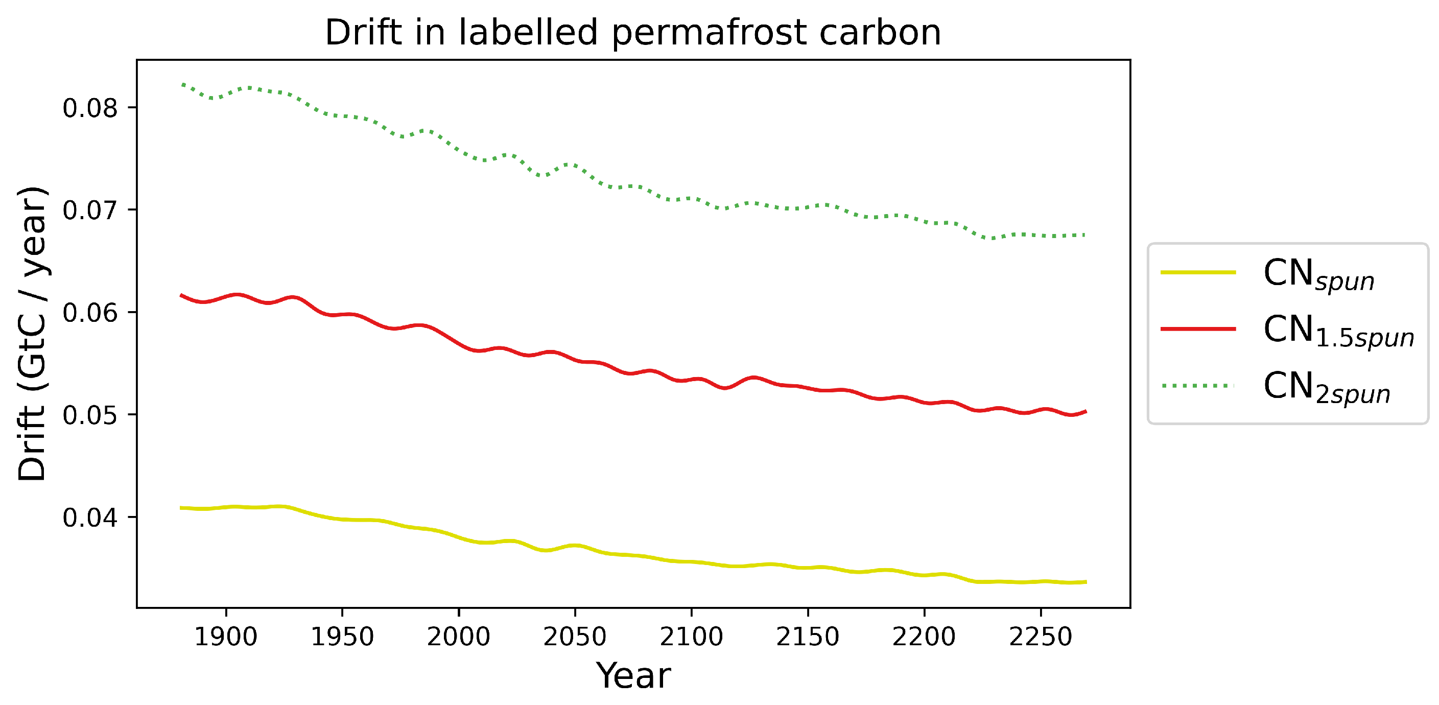
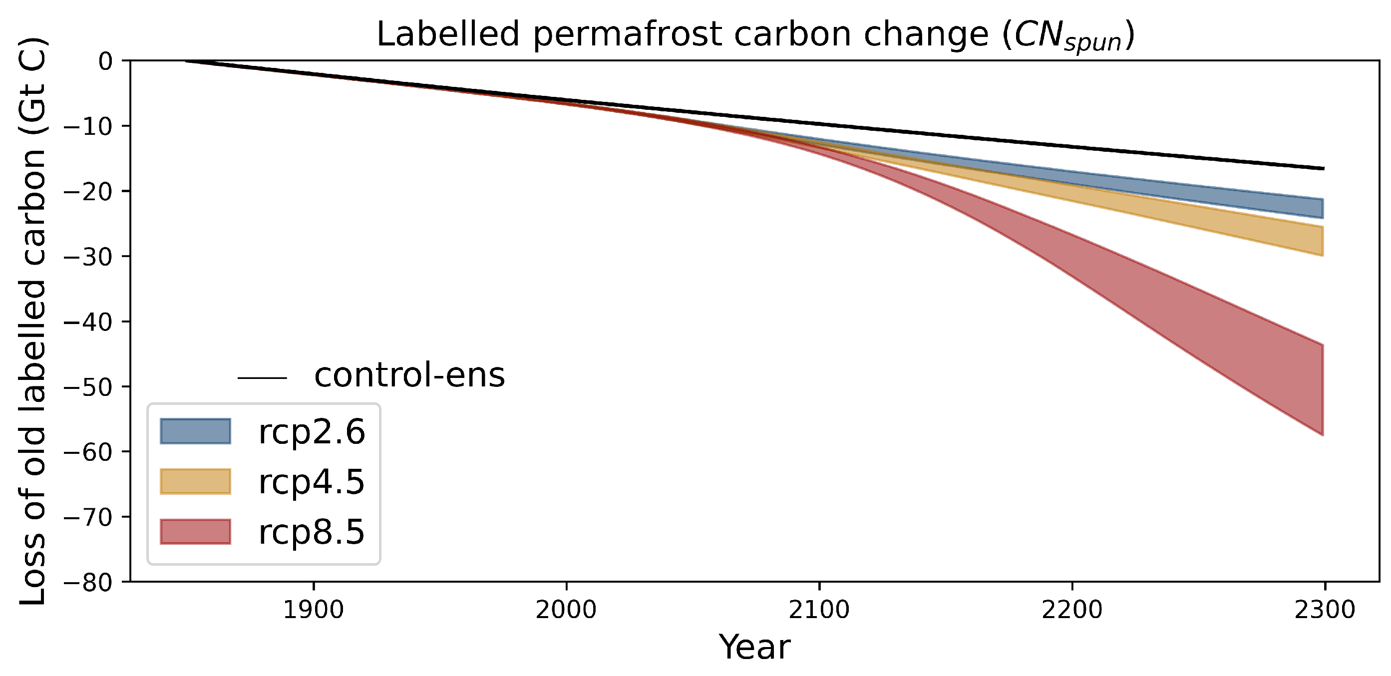
| control-ens Stationary simulations | Quantifying the non-climate related drift in permafrost C emissions.
The climate, prescribed CO emissions and N deposition are set to the values at the start of the simulation (see Section 2.1). • pfCloss is the difference in permafrost C (Gt C) between transient-ens and control-ens. |
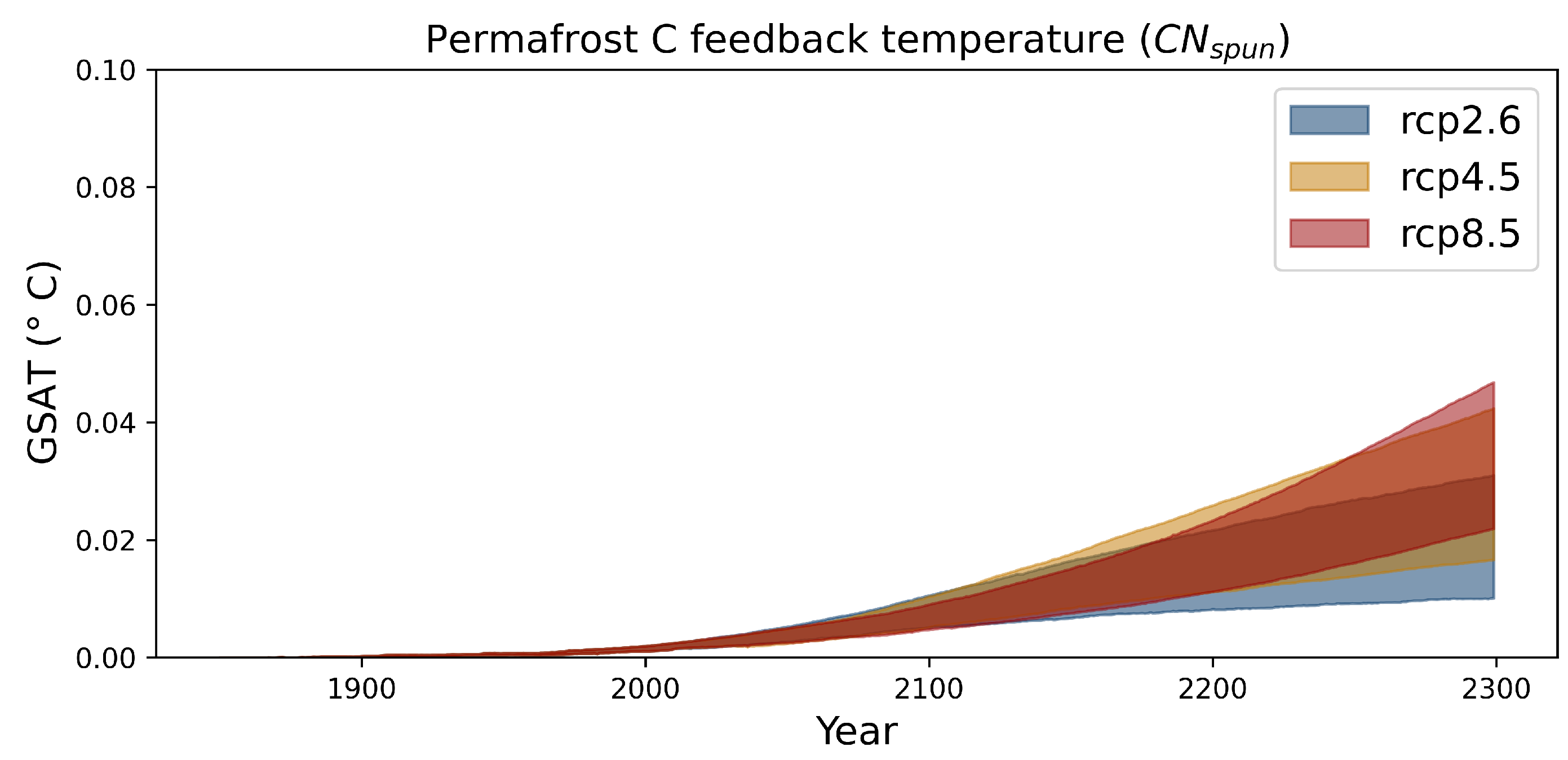
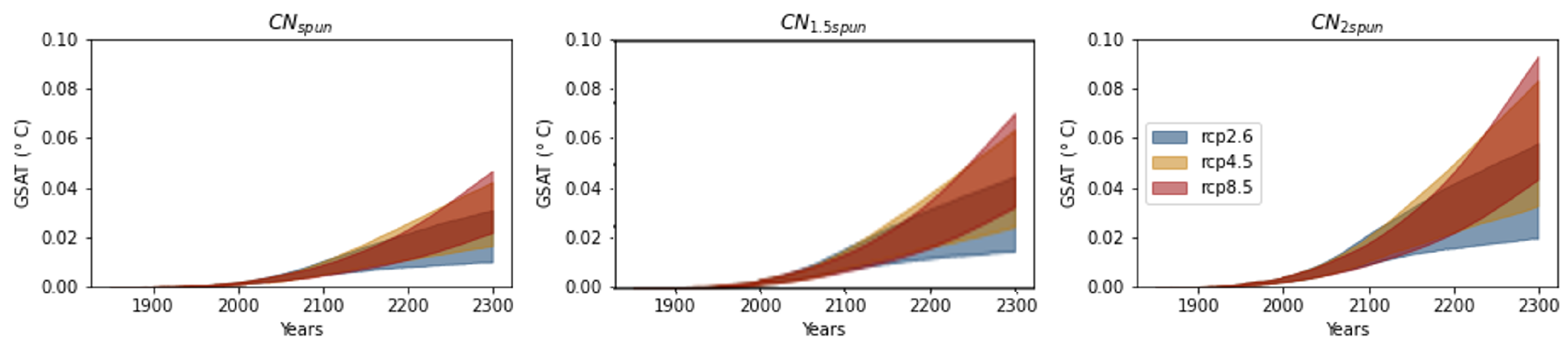
| pfCloss-feed-ens Diagnostic experiment | Quantifying the positive permafrost C feedback onto GSAT. The diagnosed permafrost C emissions from control-ens are included in the CO emissions file and only the non-permafrost C is visible to IMOGEN. • pfCloss-feed is the difference in GSAT (°C) between pfCloss-feed-ens and transient-ens. |
| Metric | Model (2000–2009) | Observed | Reference for Observed |
|---|---|---|---|
| Permafrost extent (10 km) | 15.2 | 14.3 16.2 | [1] [38] |
| Permafrost extent/ MAATC (%) | 67 | 62 71 | [1] [38] |
| Hit rate of model (%) | 50 54 | - | [1] [38] |
| Active layer thickness (m; −12 °C < MAAT < −10 °C) | 0.49 (0.42–0.65) | [42] | |
| Active layer thickness (m; −6 °C < MAAT < −4 °C) | 1.15 (0.64–1.98) | [42] | |
| Area of trees (10 km) | 2.0 | 2.9 | [43] |
| Area of grasses (10 km) | 7.1 | 3.2 | [43] |
| Area of shrubs (10 km) | 1.1 | 3.8 | [43] |
| Area of bare ground (10 km) | 4.4 | 4.5 | [43] |
| Vegetation C (Gt C) | 18.0 | 15.2 | [44] |
| Vegetation N (Gt N) | 0.1 | - | - |
| GPP (Gt C/year) | 6.6 | 5.2 | [45] |
| NPP (Gt C/year) | 3.6 | 3.0 | [46] |
| NEE (Gt C/year) | 0.20 | 0.24 | [47] |
| Ecosystem residence time (years) | 154 | 97 | [48] |
| Soil residence time (years) | 279 | 243 | [47,49] |
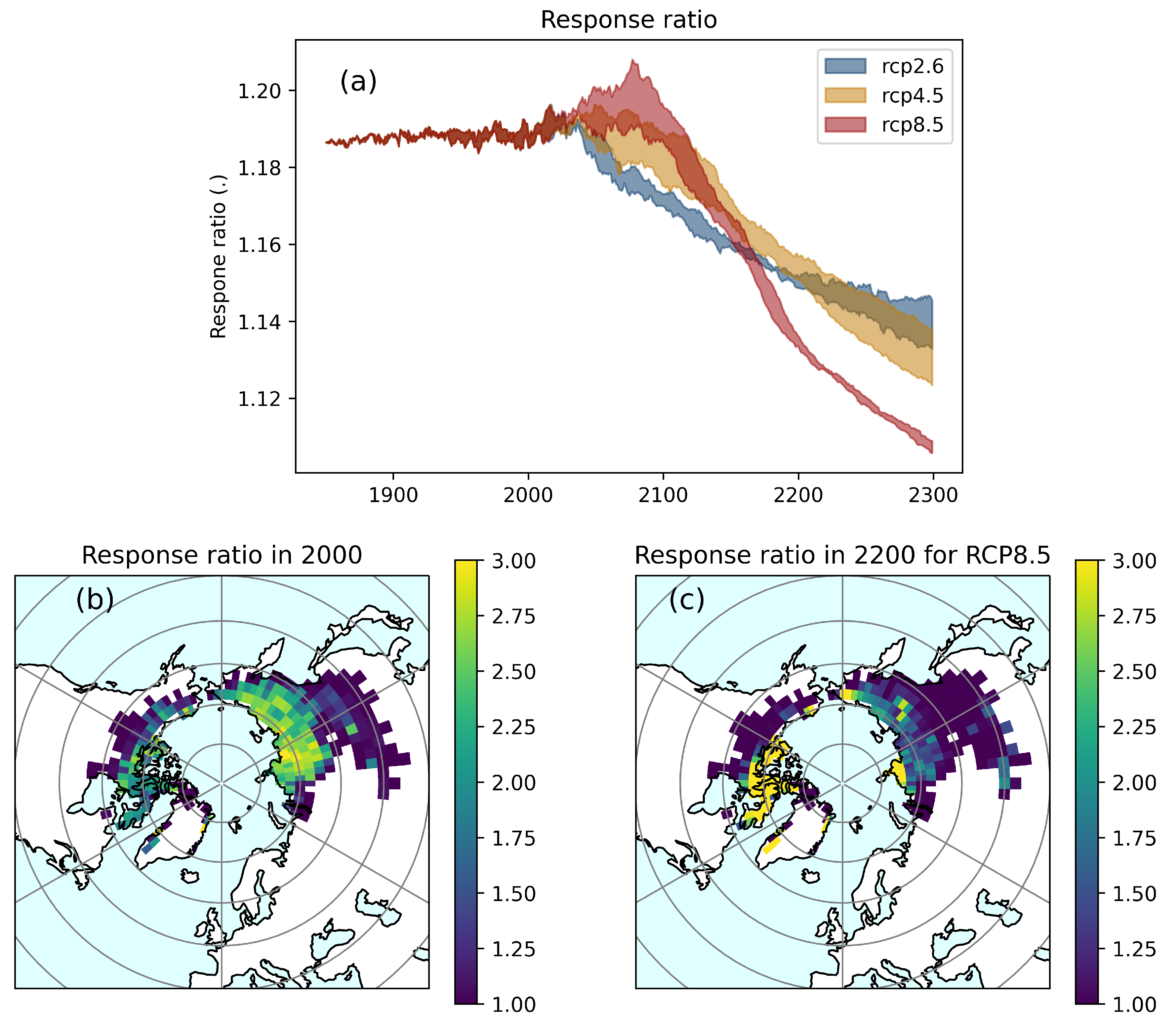
| Response ratio boreal | 1.05 | 1.20 (1.08–1.33) | [50] |
| Response ratio tundra | 1.14 | 1.35 (1.12-1.64) | [51] |
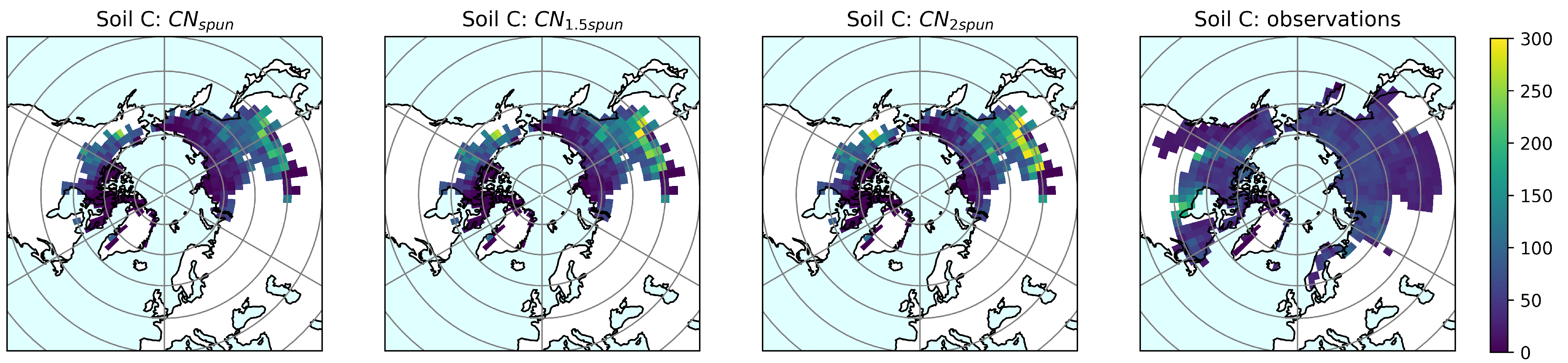
| Soil C in top 3 m of permafrost region (Gt C) | 1008 | 767 | [49] |
| Soil N in top 1 m of permafrost region (Gt N) | 664 | 24 | [52] |
| Inorganic N in top 1 m of permafrost region (Gt N) | 0.34 | - | - |
Publisher’s Note: MDPI stays neutral with regard to jurisdictional claims in published maps and institutional affiliations. |
© 2022 by the authors. Licensee MDPI, Basel, Switzerland. This article is an open access article distributed under the terms and conditions of the Creative Commons Attribution (CC BY) license (https://creativecommons.org/licenses/by/4.0/).
Share and Cite
Burke, E.; Chadburn, S.; Huntingford, C. Thawing Permafrost as a Nitrogen Fertiliser: Implications for Climate Feedbacks. Nitrogen 2022, 3, 353-375. https://doi.org/10.3390/nitrogen3020023
Burke E, Chadburn S, Huntingford C. Thawing Permafrost as a Nitrogen Fertiliser: Implications for Climate Feedbacks. Nitrogen. 2022; 3(2):353-375. https://doi.org/10.3390/nitrogen3020023
Chicago/Turabian StyleBurke, Eleanor, Sarah Chadburn, and Chris Huntingford. 2022. "Thawing Permafrost as a Nitrogen Fertiliser: Implications for Climate Feedbacks" Nitrogen 3, no. 2: 353-375. https://doi.org/10.3390/nitrogen3020023