1. Introduction
Fields are useful notions that are ubiquitous in all scientific areas. In generic terms, a field can be treated as a map** from spatial locations to a physical variable of interest. Given a reference frame, a location is specified by a set of real-valued coordinates, and the most common form of a field function is . represents the domain of the quantities of interest.
The concept of fields serves as a fundamental cornerstone in various scientific disciplines, offering a versatile framework to understand and describe diverse phenomena. Across scientific areas, field representations take on distinct forms tailored to the unique demands of each discipline. In the related physics and mathematics subjects, fields are often construed as formal mathematical entities, inviting analytical scrutiny to uncover their intricate characteristics. In the domain of quantum field theory (QFT) [
1,
2,
3], fields cease to be mere abstractions and emerge as dynamic entities permeating space and time. These fields—whether scalar, vector, or tensor—are not fixed values; instead, they are dynamic and fluctuating entities that embody the fundamental nature of quantum interactions. Transitioning from the microscopic to the macroscopic, the gravitational field introduces a different facet of field representation. In the study of gravitation [
4], fields manifest as gravitational fields, bending the geometry of space–time itself. In contrast to the analytical focus of QFT, gravitational fields lead toward a geometrical interpretation, weaving a narrative where masses dictate the curvature, and objects move along paths carved by this curvature. In applied mathematics, the study of partial differential equations (PDEs) [
5] further diversifies our perspective on field representations. PDEs are ubiquitous in describing a myriad of physical phenomena, from heat diffusion to wave propagation.
While the theoretical underpinnings of fields find elegance in formal mathematics, the practical application of field concepts in engineering demands a shift in perspective. When grappling with real-world engineering problems, computational aspects take center stage. In the area of representing and performing computations on fields, a prevalent approach involves discretization, or quantization, of space, offering a practical bridge between theory and application [
6,
7]. Depending on the application fields, various quantization schemes have been found effective. For example, Eulerian quantization [
8] finds practical application in finite element analysis, where structures are divided into smaller, discrete elements, and computations are performed at each node or element. Contrasting Eulerian quantization, Lagrangian quantization [
9] follows the motion of individual particles or elements through space and time. In simulating the behavior of fluids, Lagrangian methods track the movement of fluid particles, allowing for a detailed examination of fluid flow, turbulence, and interactions. Similarly, in simulating the dynamics of solids, Lagrangian quantization enables the study of deformations, collisions, and structural responses under varying conditions.
Recently, the development of data-driven approaches has revolutionized various scientific and engineering domains. The emergence of data-driven techniques, powered by advancements in machine learning and computational capabilities, offers a promising ability to handle complex, high-dimensional data. Specifically, a useful technique involves employing flexible parameterized representations to model the family of appropriate field functions, particularly through neural networks. Originating from computational geometry and vision, this technique aims to recover fields for subsequent computational vision tasks, such as representing light-scattering fields. Despite the rapid development of data-driven field modeling techniques, there is currently no comprehensive review summarizing the advancements in this field. Therefore, this review aims to provide an overview of state-of-the-art learnable computational models for 3D field functions. Specifically, we focus on models that utilize neural networks as function approximators, showcasing the capabilities and flexibility of neural networks in handling various fields.
The structure of this review is as follows: In
Section 2, we present the technical definition of field functions and neural networks. In
Section 3, we review neural-network-based and parametric-grid-based approximations for practical field functions. In
Section 4, we discuss the developments of the measurement process in the data-driven frameworks by reviewing existing works contributing to the observation process. This section aims to reveal the challenges in this domain and suggests emerging research problems. Finally, we conclude the review.
2. Background
A field function describes a spatially (and temporally) distributed quantity
where
represents the domain in which the interested physical process is defined, usually an extent of 3D space with an optional time span.
represents the range of the target physical properties of interest.
We consider a parameterized function space:
from which a candidate function
is selected to approximate the underlying field
f in Equation (
1). In Equation (
2),
h represents a candidate approximator for
f.
specifies a space–time point. The symbol
represents learnable parameters. There is an extra input variable to the learning field model,
, which specifies extra conditions to make observations of the underlying field (The observation condition in Equation (
2) should be considered without loss of generality. In practice, useful modeling of a physical system can be formulated by specifying the observation process. For example, a quantum mechanical system with a state vector
can often be formulated with an observation operator
).
The field model is determined in a data-driven manner. In the design stage, the parametric model family is constructed, typically by selecting a specific neural network structure. Once the network structure is fixed, specific parameter values define the particular field function. In the data-driven modeling approach, these parameters are set during an optimization process (learning). The optimization objective is formulated to ensure that the field model aligns with a set of observed variables. The modeling process involves specifying how the observable quantities used to constrain the model were generated.
Neural Networks as Function Approximator
One of the most successful families of function approximators is the neural network models [
10]. It is not surprising that multiple-layer perceptrons (MLPs) have become a prevalent framework for generic function approximation to represent a target field function. An MLP is composed of interconnected nodes, referred to as neurons, organized in layers. Each neuron is linked to every neuron in the preceding and succeeding layers. The output of a neuron is adjusted by weights and biases to approximate complex functions, allowing the capture of intricate patterns and relationships in the data.
Generally, the computation of an MLP involves multiple primary units, where, for a unit
,
where
f denotes a specific layer with input vector
. The parameters
and
determine the behavior of the particular unit.
is the activation function applied to the summation of weighted inputs and bias. This design draws inspiration from biological neurons, where synaptic weights modulate excitatory and inhibitory stimuli, akin to the weights
and bias
b in Equation (
3). The status of a neuron is determined by its response to the stimuli, akin to the activation function
. The unit in Equation (
3) is commonly referred to as a
neuron. MLP represents a specific class of computational models containing multiple units
. In an MLP, the units
are organized in an acyclic graph, and the computations are hence sorted in multiple stages. Units belonging to the same computational step, which can be evaluated simultaneously, are often referred to as forming a
layer in the network. To be specific, the inputs to a certain layer are given by:
where the superscripts on the right-hand side specifies a neural in
: the
ith neuron output in the
th layer serves as the
ith input to the neurons in the
lth layer. The inputs to the
lth layer expand recursively as in Equation (
4), and the inputs to the first layer,
, are the raw inputs of the MLP model.
MLP can serve as a generic computational model as a function approximator. Given a function
that is Borel-measurable, Hornik et al. [
10] established that for any
and for any compact subset
, there exists a two-layer neural network
f such that the supremum norm of the difference between
g and
f over
K is less than
. The neural network can be represented as:
Theoretical investigations of neural network expressivity have been conducted since then.
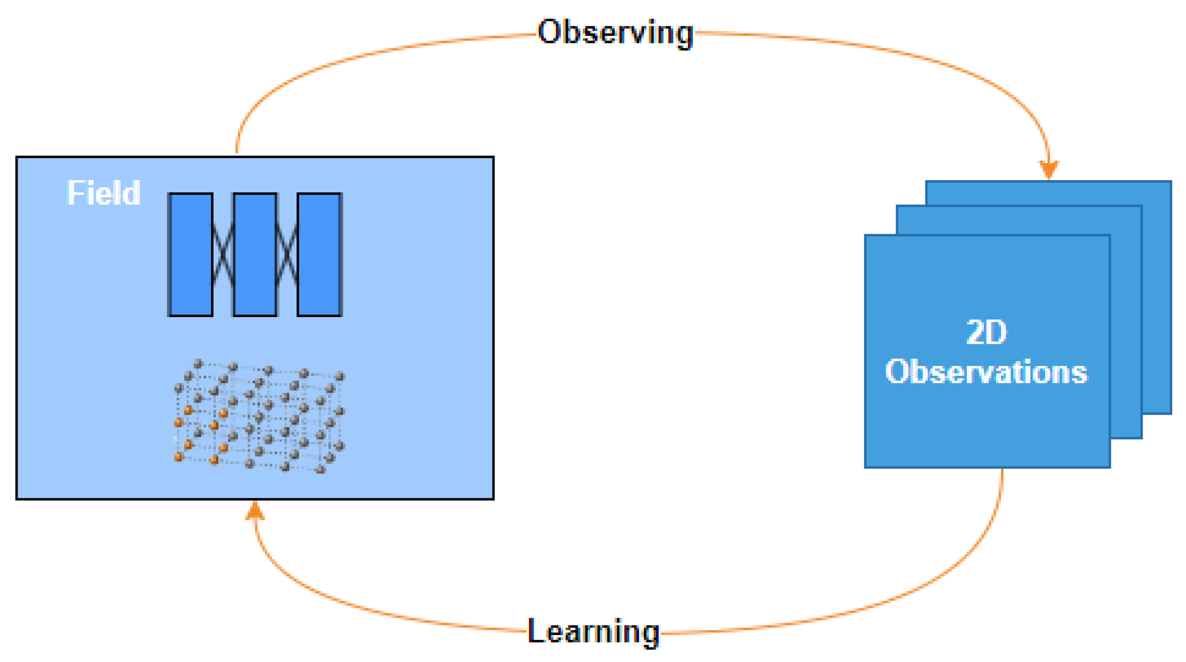
4. Computational Models of the Measurement Process
Learning models are constructed using data-driven methods. In addition to the spatial and temporal distribution of the interested physical properties, it is also necessary to incorporate the observable variables in the models, i.e., we need to describe the process of how data are measured from the physical fields, such as images from a scattering field of light. The computational observation model allows the information of the physical fields to be extracted from the sensory data and hence learn the underlying model, for example, learning a magnetic field from sensory data [
41]. In this section, we discuss several challenges and design choices in this aspect and illustrate the ideas using examples of learning light-scattering fields from sensory observations. The relationship between 2D observations and field functions is shown in
Figure 5.
Formally, recall the field approximator function family discussed in previous sections. An example instantiating Equation (
2) was discussed in
Section 3,
where
F specifies the light scattering at a location in 3D space
;
represents the observation condition of the light field, i.e., the view perspective from the two-sphere (indicating all possible viewing directions). The discussion so far focused on expressing
F in an adequate function family.
However, despite the conceptual clarity of the model, the field cannot be directly learned from measurements. In other words, a function approximation model alone cannot be used to represent practical fields. This is because learning (data-driven) models aim to find an optimal approximation to F from observations. Typically, this is achieved by minimizing the difference between the observed quantities and what the field function has specified. In the task above, actual measured sensory data are not directly related to F; instead, the data are obtained from a process of forming observations by reducing the 3D field to variables distributed on a 2D plane. The result of the observation process is 2D images.
To learn from data, constructing a computational model that mimics the process of deriving observations from the field is essential. The computational observation model facilitates inferring field information from the data. To faithfully, efficiently, and effectively formulate this process for learning, attention must be paid to several key aspects.
Specifically, we consider three aspects that underscore the significance of the observation process: the integral in 3D space, the discretization of the integral, and the diverse computational processes involved in executing the integral.
In measuring the field, quantifiable values depend on the field’s extent rather than a specific point, making direct empirical verification of field equations impractical. Thus, constructing a computational model to depict the observation process becomes necessary. Given the observational nature across a region, a logical approach is to integrate the field over that region, assuming the observation aligns with the expected value of the field function across the field.
The assumption is only valid when the interested physical quantities are reasonably homogeneous. In practical scenarios where this condition is not met, adjustments to the computational model become imperative. For instance, in the observation process within the neural radiance field, the mathematical expression involves the volumetric rendering equation, as shown in Equation (
8) [
42].
Here, the integral encapsulates the integration over the entire depth range from
to
, where
t refers to the distance between two points along a line. The variable
d corresponds to the observing direction.
is the quantity value illustrating the propensity of the volume to scatter photons—essentially, quantifying “how many” photons can be scattered. For example, a volume on the surface can scatter more photons and contribute more to the final observations.
c denotes the color at the specific position concerning observing direction.
represents the probability that photons do not contribute to the volume within the range
to
t. This introduces a probabilistic element, accounting for the likelihood that photons traverse the specified distance without interaction, formally defined as:
The computational model can be altered based on changes in the observation process. For instance, if the observation emphasizes the geometric structure of scene objects, necessary modifications to the computational model are warranted [
43,
44,
45,
46,
47,
48,
49,
50]. This might entail a transition to a model that first reconstructs the surface before undertaking the observation process [
51,
52,
53,
54,
55,
56,
57,
58,
59].
The second aspect involves the discretization process within the computational framework. A conventional method used to estimate the integral in Equation (
8) is a process known as quadrature [
24,
25,
27,
29,
30,
33,
36,
60,
61,
62,
63,
64]. This entails discretizing the continuous line into a set of discrete samples, obtained via a spatial sampler. These discrete samples function as a representative approximation of continuous volumetric data.
Specifically, in the example of NeRF, a coarse-to-fine strategy is adopted [
65]. In the coarse stage, for each line integral, a stratified sampling approach is implemented to uniformly partition the depth range [
,
] into
N bins. The mathematical definition of the sampling process within each bin is as follows:
where
represents the sampled points within each bin, ensuring a stratified distribution along the line integral. This strategic sampling approach aims to capture the varied characteristics of the scene at different depths, providing a more comprehensive representation for the subsequent integral computation.
The estimation of the integral in Equation (
8) can then be expressed in a discrete form as follows [
66]:
In this formulation, represents the estimated observing color, which is computed by summing over all the sampled points within the stratified bins. Each term in the summation accounts for the contribution of a specific sampled point i, considering its transmission probability , the volumetric scattering term , and the color value at that point. refers to the distance between adjacent samples.
Specifically, the transmission probability
is calculated using the discrete transmission function, which encapsulates the cumulative effect of volumetric absorption along the line, influencing the contribution of each sampled point to the final observation:
In the fine stage, points are sampled based on the volume that is predicted in the coarse stage, which samples more points in the regions the model expects to contain visible content. To achieve this, Equation (
9) is rewritten based on the result from the coarse stage as:
The points are then sampled based on the normalized weights: .
The sampling strategy needs to be adjusted based on different observation processes. For instance, when the integral range encompasses an unbounded scene rather than a bounded one [
67], a stratified sampling strategy may not be appropriate. In cases where the observation prioritizes the geometric structure of scene objects, the sampling strategy may have less significance in the model, given that the surface can be approximated.
4.1. Integration Adjustments
In Zhang et al. [
68], the observation model tackles the challenge regarding the scene range. In the previous discussion, Equation (
8) integrates attributes from
to
. When the dynamics range of the depth in the scene is small, a finite number of samples is enough for estimating the integral. However, when the scene is an outdoor scene or a 360-degree unbounded scene, the distance range could be large (from nearby objects to distant elements like clouds and buildings). Specifically, for expansive scenes, where distances vary significantly, the integration range becomes extensive.
The challenge arises when the observation is determined by the field evaluation over a large extent. For example, when forming images in a NeRF model, if the device is focusing outward, the distance range is large. The observation model, rooted in Equation (
8), faces complexity, as highlighted in [
68], due to the need for sufficient resolution in both foreground and background areas within the integral. However, employing a sampling strategy in a Euclidean space, as demonstrated [
23], proves challenging to meet this requirement.
Alternatively, when all cameras are forward-facing toward the scene, NeRF utilizes normalized device coordinates (NDCs) [
69] for 3D space reparameterization. While effective for forward-facing scenes, this reparameterization strategy limits possible viewpoints and is unsuitable for unbounded scenes.
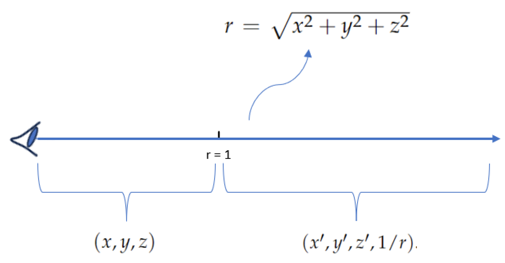
To overcome this challenge, NeRF++ [
68] employs the inverted sphere parameterization. This approach maps coordinates in Euclidean space to a new space, as illustrated in
Figure 6, offering a solution to the limitations imposed by the traditional Euclidean and NDC approaches.
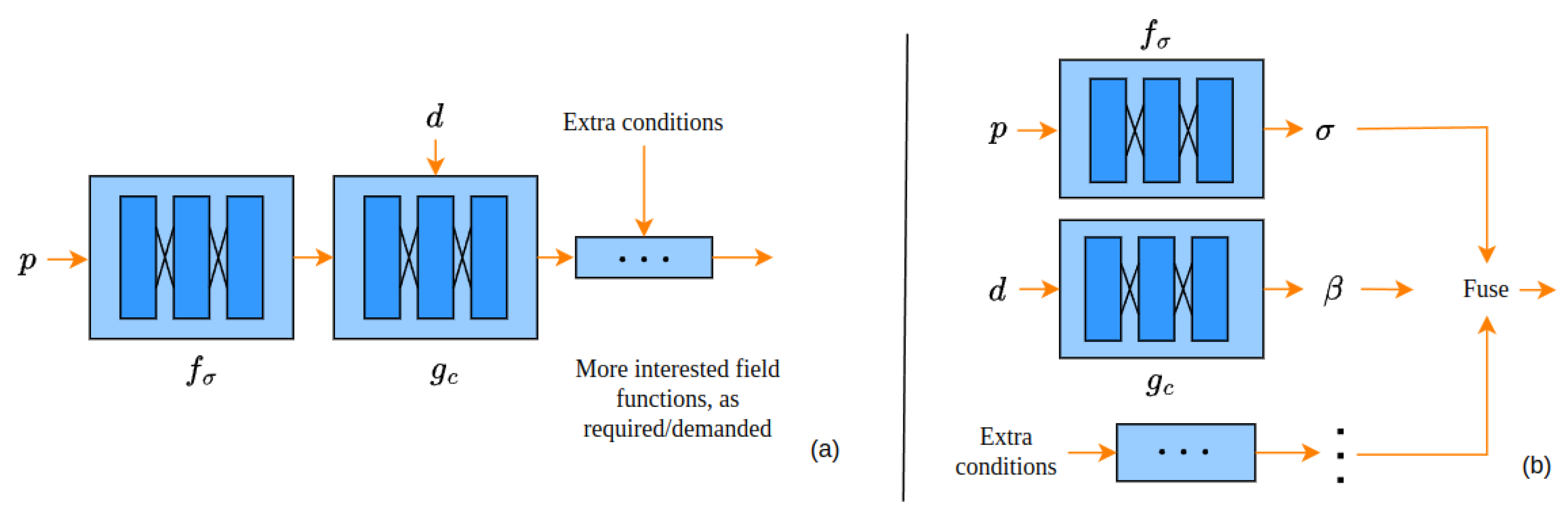
The fundamental concept behind this parameterization strategy involves a division of 3D space into two distinct regions: an inner unit sphere encapsulating the foreground and an outer space accommodating the background. The re-parameterization process is selectively applied solely in outer space. To model these two regions effectively, the framework employs two MLPs separately, each dedicated to capturing the characteristics of the inner sphere and outer space. In practical terms, to determine the color of a pixel, Equation (
4) is applied independently for the two MLPs, with the results then merged in a final composition step.
Specifically, as shown in
Figure 6, the inverted sphere parameterization in outer space reparameterizes a 3D point
, where
, into a quadruple
. The resulting unit vector
satisfies
, indicating its orientation along the same direction as the original point
and representing a direction on the sphere.
In contrast to Euclidean space, where distances can extend infinitely, the parameterized quadruple imposes bounds: , and . This finite numerical range encapsulates all values within manageable limits. Furthermore, the parameterization acknowledges that objects at greater distances should exhibit lower resolution. By incorporating into the scheme, it naturally accommodates reduced resolution for farther objects. This not only preserves the scene’s geometric characteristics but also establishes a foundation for subsequent modeling and computational processes.
With the inverted sphere parameterization, the integral Equation (
8) can be updated as follows:
where
refers to the line to be integrated;
is an observation point;
is the viewing direction.
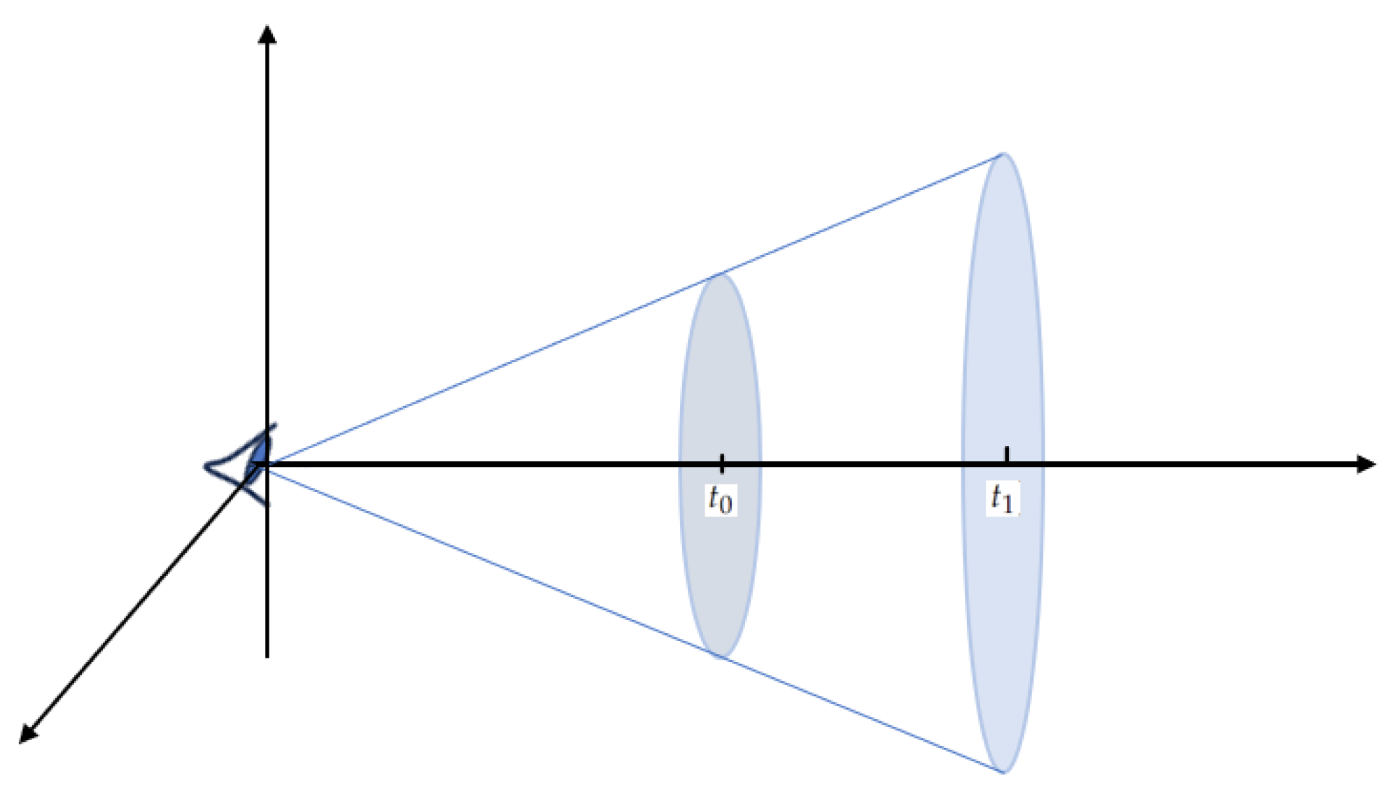
Mip-NeRF [
60] introduces a fundamental transformation to the integral process, the starting point in the computational observation process. The main change provided with Mip-NeRF is integration along 3D cones originating from each pixel instead of a line, as shown in
Figure 7. The integration along these cones captures a broader set of spatial relationships, providing a distinctive characteristic. This adjustment in the observation process results in images with reduced aliasing artifacts. By integrating along cones, Mip-NeRF extends its reach to a richer set of spatial relationships within the scene. This departure from line integration allows for a more comprehensive observation of the field representation.
Traditionally, the field was integral along each line, as shown in Equation (
8), capturing information discretely along a one-dimensional path. Mip-NeRF, however, redefines this approach by integrating along a 3D cone originating from every pixel. With the alteration from line to cone, the subsequent point sampling process undergoes a corresponding shift. Instead of uniformly sampling points along a line, Mip-NeRF adapts its sampling strategy to efficiently capture information within these 3D cones. This adjustment is reflected in the use of multivariate Gaussian distributions to approximate intervals within the conical frustums. Additionally, instead of map** a point in 3D space to a positional encoding feature, Mip-NeRF maps each conical frustum to an integrated positional encoding (IPE).
The discretization process of Mip-NeRF involves dividing the cast cone into a series of conical frustums, essentially cones cut perpendicular to their axis. However, the utilization of a 3D conical frustum as input is not a straightforward task. To address this challenge, Mip-NeRF employs a multivariate Gaussian to adeptly approximate the characteristics of the conical frustum. A Gaussian is employed to fully characterize the conical frustum with three essential values: the mean distance along the line
, the variance along the line
, and the variance perpendicular to the line
. A midpoint
and a half-width
are utilized to parameterize the quantities. This process is as follows:
where
and
correspond to the start and end depth of a conical frustum, as shown in
Figure 7, and
r refers to the width of the pixel in world coordinates scaled by
.
Crucially, as shown in Equations (
10) and (
11), the coordinate frame of the conical frustum, now represented by the Gaussian, transforms world coordinates. After the coordination transformation, IPE is applied to obtain the encoding of each conical frustum. Since this is not our focus, we do not provide further details here.
In the earlier discussion, the field measuring process was designed around the distribution of physical properties. Conversely, when the observation emphasizes the geometric structure of scene objects, necessary adjustments should be implemented in the computational model. When observing a field with a specified surface, leveraging geometric information can improve the accuracy of the observation.
An example in the radiance field is the NeuS model and its follow-ups [
43,
70,
71,
72,
73,
74,
75,
76,
77,
78]. NeuS extracts the surface by approximating a signed distance function (SDF) in the radiance field. With the extracted surface, the observation process is different from that of the original NeRF.
Before delving into the measuring process in NeuS, it is crucial to comprehend how a surface is represented in the radiance field. The surface
S of the objects in a scene is represented by a zero-level set of its SDF. As previously mentioned,
in Equation (
8) denotes the quantity value illustrating the volume’s propensity to scatter photons. For surface reconstruction, NeuS introduces a weight function
that signifies the contribution of a point’s color to the final color of a pixel by combining
and
T. The measuring process can then be expressed as Equation (
12). NeuS asserts that the weight function should satisfy two conditions for surface approximation: unbiased and occlusion-aware.
The “unbiased” criterion necessitates a weight function that ensures the intersection of the integrating line with the zero-level set of the SDF contributes the most to the pixel color. The “occlusion-aware” property of the weight function requires that when a ray passes multiple surfaces sequentially, the integration process correctly utilizes the color of the surface nearest to the device to compute the output color. NeuS formulates the weight function as Equation (
13) to make the function unbiased in the first-order approximation of the SDF.
where
refers to a point in an integral line.
To render the weight function occlusion-aware, NeuS introduces an opaque density function
to replace
in the standard observation process. The weight function can then be expressed as follows:
By combining Equations (
13)–(
15),
can be obtained:
4.2. Discretization of the Integration
As mentioned previously, NeRF++ proposes a reparameterization strategy achieved by extending the concepts in NDC to handle unbounded scenes. However, the efficacy of this strategy relies on points sampled from a one-dimensional line. With Mip-NeRF, this line evolves into a 3D cone, necessitating an extension from NeRF++’s original parameterization. The challenge arises because the reparameterization strategy designed by NeRF++ is not straightforward for the extended line-to-cone transition in Mip-NeRF. In response to this challenge, Mip-NeRF360 [
67] introduces a parameterization strategy and a sampling scheme. Departing from the conventional approach of NeRF++, this strategy harmonizes with the 3D cone structure, offering an adaptive and optimized strategy for sampling distances, extending the integral range compared with that of Mip-NeRF.
Technically, Mip-NeRF360 contributes to the observation model in two main aspects. Firstly, it introduces a parameterization method for the 3D scene, map** 3D coordinates to an alternate domain. Secondly, it provides an approach for sampling t in the discretization process.
To achieve Gaussian reparameterization, Mip-NeRF360 leverages the classical extended Kalman filter. The coordinate transformation is outlined in Equation (
16). Applying this operator to a 3D space maps the coordinates of an unbounded scene to a ball with a radius of two. Similar to NeRF++, points within a radius of one remain unaffected by this transformation.
Additionally, the sampling scheme is designed by introducing a parameterization in the 3D space. In a bounded scene, NeRF employs uniform point sampling from the near to far planes during the coarse stage. When employingn NDC parameterization, the uniformly spaced series of samples in the sampling process becomes uniformly spaced in inverse depth, fitting well with forward-facing scenes. However, this approach proves unsuitable for an unbounded scene in all directions. Therefore, Mip-NeRF360 suggests a sampling strategy, linearly sampling distances
t in disparity, as proposed by Mildenhall et al. [
79]. Barron et al. achieved this by map** the Euclidean distance
t to another distance
s, establishing the relationship as follows:
where
represents an invertible scalar function. To attain samples that are linearly distributed in disparity within the
t space, Mip-NeRF360 chooses
. This choice ensures that the samples become uniformly distributed in
s space.
In practical implementations, Mip-NeRF360 modifies the coarse-to-fine sampling strategy. Unlike NeRF, which calculates weights based on coarse-stage results and subsequently utilizes them repeatedly in the fine-stage sampling procedure, Mip-NeRF360 adopts a distinct approach. It recommends incorporating an additional MLP exclusively for predicting weights, excluding color prediction. The predicted weights are then used to sample s intervals.
Significantly, the supplementary MLP in Mip-NeRF360 is smaller than the NeRF MLP, specifically designed to constrain the weights generated by the NeRF MLP. As a result, the resampling process in Mip-NeRF360 involves reduced computational complexity compared to NeRF, owing to the considerably smaller size of the additional MLP compared to the entirety of the NeRF MLP.
4.3. Computational Process of Summing over Sampled Points
Numerical integration is commonly used for computing integrals in practice, including Riemann sums, quadratures, or Monte Carlo methods [
80]. Based on these, authors [
61] introduced a framework called AutoInt, which utilizes neural networks to approximate integrals in the evaluation stage. As shown in Equation (
8), the integral involves two nested integrations: line integration and transmission, Equation (
4), which is not trivial to approximate. Therefore, AutoInt divides each line into piecewise sections. Following this division, the observing integral can be refined as follows:
where
where
is the length of each section. After dividing the line into sections, AutoInt is applied to evaluate each integral.


