A Comprehensive TCO Evaluation Method for Electric Bus Systems Based on Discrete-Event Simulation Including Bus Scheduling and Charging Infrastructure Optimisation

Abstract

Bus operators around the world are facing the transformation of their fleets from fossil-fuelled to electric buses. Two technologies prevail: Depot charging and opportunity charging at terminal stops. Total cost of ownership (TCO) is an important metric for the decision between the two technologies; however, most TCO studies for electric bus systems rely on generalised route data and simplifying assumptions that may not reflect local conditions. In particular, the need to reschedule vehicle operations to satisfy electric buses’ range and charging time constraints is commonly disregarded. We present a simulation tool based on discrete-event simulation to determine the vehicle, charging infrastructure, energy and staff demand required to electrify real-world bus networks. These results are then passed to a TCO model. A greedy scheduling algorithm is developed to plan vehicle schedules suitable for electric buses. Scheduling and simulation are coupled with a genetic algorithm to determine cost-optimised charging locations for opportunity charging. A case study is carried out in which we analyse the electrification of a metropolitan bus network consisting of 39 lines with 4748 passenger trips per day. The results generally favour opportunity charging over depot charging in terms of TCO; however, under some circumstances, the technologies are on par. This emphasises the need for a detailed analysis of the local bus network in order to make an informed procurement decision.

1. Introduction

Municipal governments and public transport operators around the world have committed to transforming their fossil-fuelled bus fleets to zero-emission fleets, using either battery electric or fuel cell electric buses. The choice of technology has profound implications on the operational characteristics of the vehicles and the infrastructure required.

In recent years, significantly more battery electric buses were deployed than fuel cell buses, and the majority of bus operators in Europe appears to strategically favour this technology [1]. We therefore focus on battery electric buses in this work. However, even within the realm of battery electric buses, several charging strategies exist with vastly different operational characteristics (Figure 1). We differentiate between depot charging (DC), opportunity charging at stationary charging points (OC) and in-motion charging (IMC). Opportunity charging can take place at terminal stops (OC-T), intermediate stops (OC-I) and at central charging stations (OC-C).

Opportunity charging at intermediate stops (OC-I) and at central charging stations (OC-C) is rarely encountered. In Germany, for example, only two electric bus projects (out of approximately 40 in total) used OC-I, one of which has been declared obsolete [2,3]. Our interviews with bus operators also suggest that OC-I is not desired due to the complex nature of planning infrastructure on public roads. OC-C has also seen only a few applications [1]. In-motion charging (IMC) is limited to cities that already have a trolleybus network, one exception being Berlin where building new trolley bus lines with in-motion charging is currently being discussed [4]. The majority of bus electrification projects focuses on depot charging (DC) and opportunity charging at terminal stops (OC-T). Also, battery swap** exists, but it is nearly exclusively applied in China. Since our focus is on the European market, battery swap** will not be further regarded in this study.

For operators facing a decision between the two technologies, the total cost of ownership (TCO) is an important metric [5]. However, despite a wealth of publications dealing with the TCO analysis of electric bus systems, several aspects have received insufficient attention in the literature, as we will show in our literature review in Section 3 (after introducing a suitable structure for literature comparison in Section 2). In particular, many works circumvent the problem of rescheduling bus operations to satisfy the range and charging time constraints imposed by electric buses. This can lead to unrealistic results for the electric bus fleet size. The issue of increased staff demand is also commonly neglected. Most methods do not use real timetable and route data as an input, but generalised data. Delay data is not considered in any of the studies we evaluated, yet, as we will show, it has significant influence. We conclude from our literature evaluation that the existing methodologies are of limited applicability for bus operators planning the electrification of their fleet and seeking the most cost-effective option.

In Section 4 of this paper, we provide details on a simulation, planning and TCO assessment method first introduced in [6]. The method has since been further developed and currently includes

• An object-oriented, discrete-event simulation framework, enabling the energetic simulation of large bus fleets—including charging events en-route and in the depot—based on exact, non-idealised scheduling data,
• A scheduling algorithm to construct electric bus schedules adapted to range and/or charging time constraints and service delays,
• A genetic algorithm to enable cost-optimised placement of opportunity charging stations and
• A TCO calculation module based on dynamic costing.

In Section 5, we conduct a case study for a set of 39 real-world bus lines for which exact timetable, scheduling and delay data were available. By analysis of the existing (diesel bus) schedules, we will illustrate that a 1:1 exchange of diesel to electric vehicles often assumed in the literature is infeasible. We then apply the charging infrastructure optimisation and scheduling algorithms to construct fully electrified operational scenarios using depot and opportunity charging. The resulting vehicle schedules serve as input for a fleet and depot simulation that yields fleet size, fleet energy consumption, driver hours, etc. These values are then fed into the TCO module to obtain total system cost for each scenario. We close our paper with a discussion of our methodology and results (Section 6) and a final conclusion and outlook (Section 7). Detailed model equations are given in the Appendix.

2. General Workflow in Electric Bus System Planning and TCO Analysis

During recent years, an abundance of publications has emerged in the field of electric bus systems with very different scopes. Many publications focus on individual aspects of system design (for example, methods to obtain a feasible vehicle configuration or charging infrastructure layout for a given bus network) or system simulation (for example, vehicle energy consumption simulation). On the other hand, several publications deal with complete electric bus systems, mostly in order to compare different system configurations in terms of TCO. The latter studies vary considerably in the level of detail with which certain aspects are treated.

To facilitate a well-structured comparison of existing works, we propose a generalised representation of the electric bus system analysis workflow, illustrated in Figure 2. Based on comprehensive literature evaluation as well as our own developments, we identified four main steps:

• Problem formulation and input data definition
• System design methods
• System simulation methods
• TCO calculation methods.

It should be pointed out that definitions in the literature may differ. For example, in our previous work [7], the entire process consisting of steps 1 to 4 is regarded as system design. Generally, steps 2 to 4 are not semantically separated in the literature. They are also often not carried out sequentially, but simultaneously. This is especially the case in works utilising optimisation routines where some or all of the tasks are integrated into an objective function. For example, electric bus scheduling methods must incorporate some sort of vehicle model to determine energy consumption and vehicle range. In our generalised workflow, the scheduling algorithm is part of the system design methods and the vehicle model contained therein is part of the system simulation methods. This separation of design and simulation aspects enables us to systematically compare existing methodological contributions, even if scope and context of the respective publications differ.

3. Literature Review

In the following subsections, existing works corresponding to each of the four steps introduced in Section 2 will be evaluated.

3.1. Problem Formulation and Input Data Definition

Many different problem formulations related to electric buses have been addressed in the literature (some examples were provided above). The selection of input data is highly dependent on the problem formulation. For instance, vehicle configuration—in particular, battery capacity—may be fixed and thus provided as an input parameter [6,8], or it may be part of the design problem [5,7,9]. The same applies to the location of charging infrastructure. An aspect of high practical relevance is the form of vehicle operation profile that is used as an input. Various types of operation profiles are observed:

• Driving profiles, i.e., a time series of velocity and elevation. These may be measured in real-world operation [10], taken from standard dynamometer driving cycles [7,11] or generated from microscopic traffic simulation [12].
• Simplified bus line and timetable data. Real-world timetables are reduced to headway and trip duration (sometimes variable over the course of the day), neglecting absolute departure and arrival times; bus lines are commonly reduced to a single route variant [5,8,9,13,14,15]. (It is common for bus lines to have full-length services operating “from end to end” as well as services operating on a shorter route inbetween, or to have several different branches. We term each of these a route variant.) A slightly more detailed timetable representation is found in Ke et al. [16] where absolute departure times and variable trip durations are considered, but resampled to 5-minute intervals.
  Timetable data is often complemented with driving profiles to determine trip energy consumption [5,9,14,15].
• Exact bus line and timetable data. No simplifications are made to timetable data; any sequence of trips on any line and any route variant can be considered. This approach is common to all works specifically dealing with bus scheduling (see Section 3.2), but seldom encountered in electric bus TCO studies, exceptions being Rogge et al. [17], Lindgren [18] and Jefferies and Göhlich [6].
• Transportation demand data. Some publications do not assume fixed timetables, but regard the timetable as part of the design problem. They use demand data (e.g., passengers per hour) as an input [19,20].

3.2. System Design Methods

Depending on the problem description, considerably different methodologies are employed in this step. A common design task carried out in electric bus publications is to determine a feasible set of vehicle parameters, such as the battery capacity required for a given bus line [7,9,21] or a TCO-optimised battery capacity and/or charging power [22,23].

Also, various methods to determine charging infrastructure locations have been developed. They commonly use mixed-integer linear programming (MILP) and place charging infrastructure such that total system cost is minimised, for example, [24,25]. Some approaches also simultaneously determine cost-optimised battery capacities [22,23]. Lindgren [18] uses an optimisation heuristic to determine charging infrastructure locations and then sets the vehicles’ battery capacities such that a certain lifetime is achieved. However, all aforementioned methodologies assume unchanged vehicle schedules. Their applicability is therefore limited to situations where charging at intermediate stops (OC-I), or, in the case of Lindgren [18] and Liu and Song [23], in-motion charging (IMC) is allowed. If charging is only desired at terminal stops (OC-T), a feasible solution may not be found depending on the dwell times available. Kovalyov et al. [20] formulate an optimisation problem to determine cost-optimised fleet mix, departure frequencies and charging infrastructure layout; however, no implementation is provided and it is thus unknown if real-world problem instances can be solved.

If it is not possible to operate existing vehicle schedules with electric buses—due to range or charging time limitations—the issue of vehicle scheduling arises. We consider scheduling to be a central part of electric bus system design and a prerequisite for TCO analysis [6]. However, like the literature on charging infrastructure optimisation, publications dealing with electric bus TCO analysis often do not address the scheduling problem.

In TCO studies dealing with depot charging (DC), the scheduling problem is commonly circumvented by assuming that the daily distance covered by each vehicle does not exceed the electric buses’ range [11,26] or by setting a sufficiently high battery capacity, even beyond what is available on the market [13]. When treating opportunity charging (OC), the need for rescheduling is eliminated in several works by assuming charging at intermediate stops (OC-I) and deploying a sufficient amount of charging stations such that dwell times at the terminal stops can remain unchanged [5,9,13,18]. (The work by Lindgren [18] does make use of a scheduling algorithm; however, it is used to generate diesel bus schedules because original scheduling data was not available, and no details of the algorithm are given.) These assumptions result in unchanged vehicle demand compared to the existing, conventional bus fleet. However, we have previously shown this not to reflect the reality of a metropolitan bus network [6] and will further elaborate on this in Section 5.2.

The aforementioned works do not provide a solution for depot charging if schedule lengths exceed vehicle range; neither do they allow opportunity charging exclusively at terminal stops (OC-T). The work by Pihlatie et al. [26] does deal with OC-T, but assumes sufficient dwell times are available to recharge at the termini. We have also shown this assumption not to hold true in real-world bus operation, especially if service delays are taken into account [6].

We are currently aware of only two contributions (other than our own) that determine electric bus system TCO utilising electric vehicle scheduling. Rogge et al. [17] developed a genetic algorithm to determine feasible, TCO-optimised schedules for depot charging, including a charging sequence at the depot minimising vehicle and charging infrastructure demand. This method yields a set of vehicle schedules that satisfies exact, real-world timetables and therefore enables a realistic determination of the resulting fleet size. However, it is applicable to depot charging (DC) only. In the TCO study by Ke et al. [16], a scheduling algorithm for opportunity charging at central charging stations (OC-C) and depot charging (DC) is developed. Timetable data resampled to 5-minute intervals is used as an input. However, the algorithm does not consider the duration of deadhead trips—as a result, vehicles may be assigned trip sequences they cannot actually serve—and is subject to arbitrary restrictions, the rationale of which remains unexplained: Opportunity charging can take place only once an hour, and depot charging commences only after all vehicles have completed all trips.

Due to the lack of universally applicable scheduling methods found in electric bus TCO studies, we conducted a survey of publications focusing exclusively on electric bus scheduling.

Table 1. Comparison of electric bus scheduling methods. Legend: • yes; ∘ no; – not applicable; ? unclear.

Source	Optimisation	Multiple Depots	Vehicle Type Restrictions Per Trip	Charging Strategies			Route Restriction	Charging Duration Dependent on Vehicle SOC	Partial Charging Allowed	Charging Station Capacity Constraint	Depot Capacity Constraint	Variable Fleet Mix	OC Charging Location Optimisation
				DC	OC-T	OC-C
Rogge et al. [17]	•	∘	∘	•	∘	∘	energy	•	∘	–	∘	•	–
Ke et al. [16]	∘	∘	∘	•	∘	•	energy	•	∘	∘	∘	∘	∘
Jefferies and Göhlich [6]	∘	∘	•	•	•	∘	energy	•	∘	∘	∘	∘	∘
Paul and Yamada [27]	∘	–	∘	∘	•	∘	none	•	•	∘	–	•	∘
Wang and Shen [28]	•	•	∘	•	∘	∘	time	∘	–	–	•	∘	–
Li [29]	•	∘	∘	•	•	•	distance	∘	–	•	•	∘	∘
Adler and Mirchandani [30]	•	•	∘	•	•	•	energy	∘	–	∘	•	∘	∘
Wen et al. [31]	•	•	∘	•	•	•	energy	•	•	∘	∘	∘	∘
Li et al. [19]	•	•	•${}^a$	•	•	•	energy	∘	–	•	∘${}^b$	•	•
Reuer et al. [32]	•	?	∘	•	•	•	energy	∘	–	∘	?	•${}^c$	∘
van Kooten Niekerk et al. [33]	•	∘	∘	•	•	•	energy	•	•	∘	∘	∘	∘

${}^a$ This work differs from the others in that timetable creation is part of the problem formulation, so timetables are not given explicitly. In constructing the timetable, however, different vehicle capacities are considered based on passenger demand. ${}^b$ Overall fleet size constraint. ${}^c$ Mix of diesel and electric buses.

gives an overview of these works as well as those already discussed above. They are compared with respect to the following criteria:

• Whether or not an optimal solution to the vehicle scheduling problem (VSP) is sought (column ”optimisation”).
• The ability to handle multiple depots.
• The ability to specify vehicle type restrictions for each trip. This is highly relevant to practical operation as different trips are often served by different vehicle types (e.g., small or large vehicles).
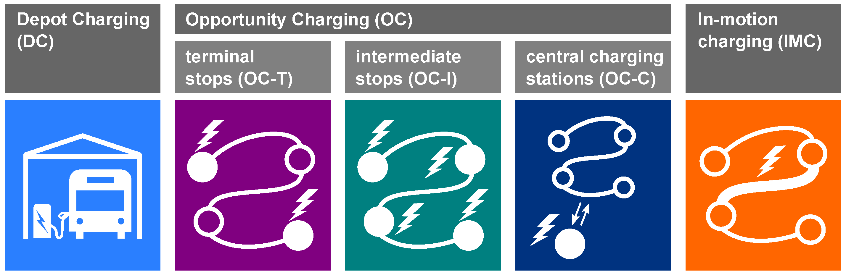
• The charging strategies considered (see Section 1 for their respective definitions).
• Whether route restrictions are imposed in terms of energy (i.e., battery capacity), time or distance.
• Whether charging duration is evaluated based on the actual vehicle state of charge (SOC) or assumed constant.
• Whether partial charging is allowed or a full charge is assumed at each charging event.
• Whether charging stations and/or depots have a limited number of charging points (capacity constraints).
• Whether a variable fleet mix is determined, for example, an optimal combination of short-range and long-range electric buses or an optimal combination of diesel and electric buses.
• Whether or not the approach determines the optimal location of OC charging stations (OC charging location optimisation).

Most works focus on finding an optimal solution to the VSP, which, when considering battery capacity limitations, is NP-hard [29]. The central task in solving such problems is to develop feasible solution heuristics. Discussing these solution procedures is beyond the scope of this paper; it should be noted, however, that application is not always proven for large problem instances of several thousand trips. For example, the time-space-energy network approach by Li et al. [19]—the approach in Table 1 with the most general problem formulation—was not able to solve an instance consisting of a comparatively small route network with four terminal stops, despite time being discretised to 30-minute intervals. The methods by Wen et al. [31] and van Kooten Niekerk et al. [33] were successfully applied to instances with around 500 trips, the method by Li [29] to around 900 trips. Adler and Mirchandani [30] demonstrated successful application for over 4000 trips and Reuer et al. [32] for over 10,000 trips.

The approaches by Ke et al. [16], Paul and Yamada [27] as well as our own [6] employ greedy algorithms and therefore do not yield optimal solutions, but are considerably less cumbersome to implement than optimisation methods and provide fast results even for very large problem instances. They are, however, applicable only to single-depot problems and are limited to DC and OC-T charging strategies.

As mentioned above, the ability to consider different vehicle types in the timetable is of great significance for real-world applications. Most works, however, do not enable this and would therefore require generating a separate problem instance for each vehicle type. This would provide feasible results only if capacity constraints and charging location optimisation are not part of the problem.

3.3. System Simulation Methods

In this section, existing methods for vehicle, fleet and depot simulation are compared.

3.3.1. Vehicle Modelling

Traction energy consumption is commonly determined by one of three approaches. Some works employ a longitudinal dynamics model comprising a detailed representation of the vehicle drivetrain [9,10,14,15,17,34,35]. A driving profile (see Section 3.1) is required as an input to the model. Others use empirical correlations describing traction consumption as a function of, for example, average velocity, eliminating the need for driving profiles [5,8]. The most simple approach to traction modelling is to assume constant specific consumption (e.g., in kWh/km) irrespective of the actual driving profile [6,13,16].

The heating, ventilation and air-conditioning (HVAC) system is the most energy-consuming auxiliary device in an electric bus, its consumption potentially exceeding that of the drivetrain depending on weather conditions [7]. Despite this, most works related to electric bus system analysis and design do not model the HVAC system explicitly. Sebastiani et al. [15] do not consider the HVAC system at all. Hegazy et al. [35] perform vehicle simulations for various auxiliary powers, but they are not linked to a specific choice of an HVAC system or specific weather conditions. Several authors use average overall vehicle consumption values, but do not state whether they include auxiliary consumption [8,13,16]. Lajunen [9] employs HVAC consumption data from Lajunen and Kalttonen [36], but it is unclear how the values were determined. Rogge et al. [17] employ a vehicle model from Sinhuber et al. [34] which uses measured values for auxiliary consumption (including the HVAC system). A detailed standalone HVAC system model was developed by the authors of this work [37,38]; however, its complexity impedes application within a fleet model. Kunith [5] uses this model to compute HVAC consumption for selected ambient temperatures prior to fleet simulation.

Explicit modelling of other auxiliaries in electric buses, such as air compressor, steering pump and battery heating/cooling, is—to the best of our knowledge—not encountered in the literature within the context of electric bus system analysis and design.

3.3.2. Fleet Modelling

We distinguish between two approaches to fleet simulation. Object-oriented or agent-based models using a discrete-event framework were popularised in autonomous taxi fleet and general logistics simulation [39,40,41,42], but are also applied to bus fleets [14,15,43,44]. All objects in the simulation—vehicles, charging stations, depots, etc.—are simulated simultaneously in a shared environment with a central simulation clock, each object having its own individual state. Events change the system state at discrete time steps and allow for communication between objects. The second approach is sequential models in which vehicles do not share an environment and each vehicle’s state is evaluated separately [10,16,17]. Some models assume that all vehicles have a uniform operation profile [5,8,9,13], hence only one vehicle is evaluated and its energy consumption is multiplied by the fleet size.

3.3.3. Depot Modelling

Especially in the case of depot charging, the charging process at the bus depot can be a bottleneck with major influence on the e-bus fleet size (and therefore on TCO), as we will show in Section 5.4. Several TCO studies, however, do not consider depot operations at all [8,9,13]. Some works approximate the additional vehicle demand arising from exchanging buses with depleted battery capacity and recharging them at the depot [5,45], but this specific approach is only applicable when using simplified timetable and route data (assuming constant travel duration and headway all day).

Rogge et al. [17] already consider the depot charging process at the scheduling stage (see Section 3.2); hence, its influence on fleet size is accounted for. However, as mentioned above, the methodology cannot handle opportunity charging.

A comprehensive electric bus depot model applicable to real-world bus schedules and any charging strategy is presented by Lauth et al. [46]. It is based on discrete-event simulation and considers all relevant processes at the depot, including cleaning, maintenance, parking, charging and dispatch.

3.4. TCO Calculation Methods

TCO calculation may be carried out on the basis of a static [8,16,17] or dynamic [5,9,13] costing model. Static models assume a constant value of money over time, while dynamic models operate in terms of net present value (NPV). Usually, dynamic models also feature cost projections for future expenditures.

Aside from the type of costing model, the existing TCO studies also vary in the selection of cost components. While all studies include vehicle and infrastructure investment cost and energy cost, the following cost components are not always accounted for: financing, driver wages, grid connection, vehicle and infrastructure maintenance, carbon emissions, salvage values.

3.5. Comparison of Electric Bus TCO Studies

Following our survey of individual methodological contributions to electric bus system design, simulation and TCO calculation, we will now analyse existing TCO studies that compare electric bus systems in their entirety.

Table 2. Comparison of electric bus system TCO studies. Legend: • yes; ∘ no; – not applicable; ? unclear.

Source	ChargingStrategies	Exact Timetables	Delays	Fleet SizeCalculation		ChargingInfrastructureDemand Calculation	Staff Demand Calc.
				E-Scheduling	Depot
Fusco et al. [8]	OC-I, OC-T	∘	•${}^a$	approx.	∘	heuristic	∘
Bi et al. [13]	DC, OC-I	∘	∘	none	∘	?	∘
Jefferies and Göhlich [6]	DC, OC-T	•	•	exact	•	heuristic	•
Kunith [5]	DC, OC-I	∘	∘	approx. ${}^b$	approx. ${}^c$	optimisation ${}^d$	partly ${}^e$
Rogge et al. [17]	DC	•	∘	exact ${}^f$	•	optimisation ${}^g$	•
Ke et al. [16]	DC, OC-T	•${}^h$	∘	approx. ${}^i$	•	?	∘
Lajunen [9]	DC, OC-I, OC-T	∘	∘	?	∘	heuristic	∘
Lindgren [18]	OC-I, IMC	•	∘	none	∘	optimisation	∘
Vilppo and Markkula [21]	OC-T	∘	∘	none	∘	heuristic	∘
Pihlatie et al. [26]	DC, OC-T	∘	∘	none	∘	heuristic	∘

${}^a$ Delays are considered implicitly by measurement of real trip durations. ${}^b$ For depot charging (DC) only. ${}^c$ For DC only. ${}^d$ Optimisation using mixed-integer linear programming (MILP) model. ${}^e$ Only additional staff demand for DC. ${}^f$ Full scheduling with genetic optimisation. ${}^g$ Optimisation using MILP model. ${}^h$ Timetables are resampled to 5-minute intervals, but it may be assumed that the model can also operate with higher resolution data. ${}^i$ Simplified scheduling without deadheading.

lists some features of electric bus TCO studies:

• The charging strategies considered,
• Whether exact timetable data is used as input,
• Whether delays are considered during system design,
• Whether bus scheduling is performed for fleet size calculation and in what manner,
• Whether charging at the depot is considered for fleet size calculation,
• How the location and/or number of required charging points is determined,
• Whether staff (i.e., driver) demand is part of the calculation.

The majority of the works uses simplified scheduling or no scheduling at all. As a consequence, application of these methods is limited to theoretical cases where the existing schedules do not have to be changed for electrification (see Section 3.2). Also, most works cannot operate on real-world timetable data, do not consider operational delays, and do not consider the charging process at the depot for fleet size calculation. The only work to feature an exact approach to scheduling and depot operations (Rogge et al. [17]) can treat depot charging only.

For a bus operator facing a procurement decision between various electric bus system alternatives, it is desirable to determine the TCO of each electric bus system for the local operating conditions, i.e., the exact local routes and timetables, rather than for generalised or simplified cases that may not adequately reflect local conditions. We must conclude, however, that none of the methods discussed in this section can deliver this.

4. Electric Bus System Simulation and Planning Tool

To be able to perform a TCO comparison of electric bus systems for a real-world, metropolitan bus network, we developed eFLIPS (Electric Fleet and Infrastructure Planning/Simulation), a simulation and planning tool first presented in [6]. It alleviates most of the limitations of existing methods discussed in the previous section: It operates on the basis of exact timetable and delay data; vehicle operations are rescheduled to account for range and charging time limitations; individual vehicle states are traced; it includes operations at the depot when determining fleet size; it enables the use of detailed vehicle consumption models. Development took place in multiple projects, not only in the context of electric buses, but also battery-electric trains and electric sanitation vehicles.

eFLIPS was implemented in Python [47] using strict object orientation. A discrete-event simulation framework was built using SimPy [48], a package providing a simulation clock, an event and process system, and capacity-constrained resources. Figure 3 gives an overview of the tool’s main features, the workflow involved in performing a TCO study as well as the inputs and outputs of each step. Each of the features will be explained in the following.

4.1. Bus Scheduling Algorithm

Our scheduling algorithm can plan schedules for depot charging (DC) and opportunity charging at terminal stops (OC-T). It follows a greedy approach similar to Paul and Yamada [27], but provides more flexibility: It can handle multiple vehicle types; it is possible to plan schedules for depot charging or refuelling; in the case of opportunity charging, charging is not assumed at every terminus, but only at those stops defined as charging points. Like the algorithm by Paul and Yamada [27], it is limited to a single depot.

The main input to the algorithm is a timetable, i.e., a list of passenger trips sorted by departure time. A trip has the following attributes: trip type (passenger or deadhead trip); vehicle type (e.g., standard or articulated bus); departure time; trip duration; delay; dwell time succeeding the trip (at this stage, the dwell time is unknown and thus set to zero). Also, a list of charging locations and a set of vehicle parameters must be provided. The output is a list of schedules, which, essentially, are also lists of trips, except they include deadhead trips and must only consist of trips of identical vehicle type.

The algorithm operates in two stages: First, schedules are built from successive trips without deadheading (other than the depot trips at the start and end of the schedule), i.e., the next trip must always begin at the destination of the previous. If the destination is a charging point, sufficient dwell time is provided to fully recharge the energy storage before the next trip commences. A global minimum dwell time can be specified. Optionally, delays can be added to the dwell time to ensure sufficient charging time and punctuality. After the addition of each trip, the vehicle SOC is evaluated. A schedule is terminated if one of the following is true: There are no more serviceable trips from the current destination (either no trips with a matching vehicle type are left at all, or those that are left exceed the maximum permitted dwell time); or, a critical state of charge is reached. In the latter case, trips are subsequently removed from the end of the schedule until the state of charge is valid. Figure A1 in Appendix A shows a flowchart of this stage of the algorithm.

In the second stage, depicted as a flowchart in Figure A2 (Appendix A), it is attempted to concatenate the schedules created in stage I in order to maximise schedule length and to avoid unnecessary trips to the depot. The algorithm tries to join each schedule with the earliest reachable follow-up schedule through a deadhead trip until no more reachable schedules exist or a critical SOC is encountered. Similarly to stage I, the duration of the deadhead trip and the subsequent dwell time are capped to avoid excessive dwelling.

The distance of deadhead trips, i.e., depot trips and trips connecting different schedules, is determined through the openrouteservice car routing API [49]. A constant average speed is assumed to determine the duration of deadhead trips. For each of the two scheduling stages, it is possible to allow or disallow line changes.

4.2. Schedule Simulation

The schedule simulation forms the main component of eFLIPS. It enables simulation of any kind of predefined schedules using one of the four charging regimes introduced in Section 1.

As pointed out above, the implementation follows an object-oriented approach. Thus, a schedule simulation replicates the physical objects encountered in the real world as depicted in Figure 4:

• A list of schedules to be served is provided, as well as the geographical grid comprising grid points and connecting arcs. Typically, the schedules cover a single operational day, but any time window up to a week is possible.
• The ambient (omitted in Figure 4) provides ambient temperature and insolation.
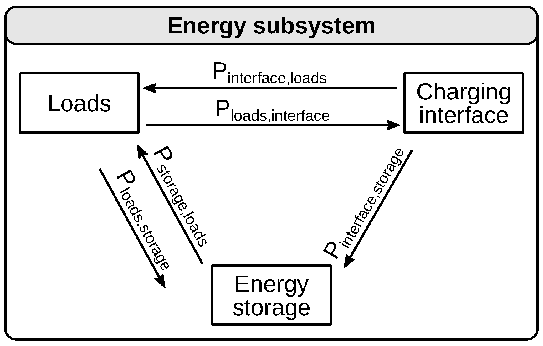
• The charging network consists of charging points for stationary charging and charging arcs where vehicles can charge while in motion. Points and arcs each correspond to a point or arc in the grid, respectively. Charging facilities have a specific charging interface through which they can transfer energy to a vehicle. They are implemented as a SimPy resource with a defined capacity (i.e., the number of charging slots available). If a vehicle issues a charging request and all slots are occupied, it must queue for a free slot in order to charge.
• One or more depots exist where vehicles start and end their respective schedules.
• A central dispatcher reads the list of schedules and, when a schedule is about to commence, requests a vehicle of the required type from the depot specified in the schedule. It also assigns a driver to the vehicle.
• Each vehicle provides various actions: Switching the ignition and air-conditioning on and off, driving along a specified leg of a schedule, driving along a specified velocity profile, modifying the payload (through boarding and alighting of passengers), etc. It has several sub-components, mainly the traction device, auxiliary devices and energy storage, as well as one or more charging interfaces. The vehicle model is explained in detail in Section 4.2.2 and Appendix C.
• The driver executes vehicle actions according to the schedule. It also keeps track of the time spent driving and idling.

A formal listing of all inputs to the schedule simulation is given in Appendix B.

4.2.1. Discrete-Event Simulation Framework

The discrete-event system allows for communication between objects. For example, if a vehicle’s traction power changes, the traction device triggers a state change event. The vehicle’s charge controller listens for state change events and, upon receiving such an event, updates the energy flow to or from the energy storage. Similarly, charging facilities keep track of the total energy flow and the number of vehicles present. State change events also control when an object’s state is logged by the data logging system: The state of any object is only evaluated when it changes, saving computing time and memory.

4.2.2. Vehicle Model

A vehicle comprises a primary and, optionally, a secondary energy subsystem, each consisting of an energy storage, any number of connected devices (loads)—including traction, HVAC and other auxiliary devices—and any number of charging or refuelling interfaces. A charge controller routes the energy flow between loads, storage and interfaces. Upon each state change event, the energy storage integrates the net energy flow to determine the amount of energy charged or discharged. The structure of the vehicle and energy subsystem models is shown in Figure 5. The primary subsystem always includes the traction motor; a secondary subsystem may be present, for example, if the heating system uses a different fuel than the traction motor, as is the case in electric buses with diesel-fueled heating.

Two traction models are available for simulation (cf. Section 3.3.1): A constant specific consumption model that determines energy consumption on a per-arc basis, and a longitudinal dynamics model requiring a driving profile. The latter currently cannot be used for schedule simulation, however it is used to determine typical mean consumption values for standard driving cycles that can later be used in a schedule simulation.

Several HVAC component models were implemented using parameters from manufacturers’ data: Electric heat pump, electric air conditioning, electric resistance heater and diesel heater can be combined to several HVAC system configurations. Auxiliaries other than the HVAC system are modelled as one device with constant power.

A charging logic checks for the availability of suitable charging facilities at the current location during every time interval and controls the vehicle’s behaviour accordingly. The actions invoked by the charging logic are depicted in Figure 6. Queueing and manoeuvring are generally only applicable to stationary charging points. Various queueing strategies can be defined: Vehicles can queue for a free charging slot or skip charging if all slots are occupied; also, vehicles can release the charging slot once they are fully charged, or remain at the charging point until departure. These features were implemented to be able to evaluate the impact of different driver break regulations on charging infrastructure demand. It is also possible to force vehicles to always wait until fully charged (even if this causes a delay), or to depart as punctually as possible (even if this leaves no time to charge).

Furthermore, several energy storage (battery, diesel tank) and charging interface models (stationary pantograph, trolleybus pantograph, CCS plug, diesel nozzle, train pantograph) were implemented. When connected to a charging interface, a constant charging power is assumed.

A full documentation of the model equations is given in Appendix C.

4.2.3. Depot Model

Vehicles start and end their schedules at a depot. Any number of depots can be defined in the simulation. Each depot keeps track of the number of vehicles currently in service and the number of vehicles present at the depot for charging and parking. All depots are empty at the start of the simulation. If a vehicle is requested for line service from a depot by the dispatcher, the first available vehicle currently parked at the depot is chosen; if no vehicle is available, a new vehicle is generated and added to the depot. Thus, the required fleet size can be determined by counting the number of vehicles generated in total by the end of the simulation, as illustrated schematically in Figure 7.

When a vehicle arrives at the depot and a charging slot is available, charging commences immediately after a defined dead time for manoeuvring has passed. Vehicles are charged at full power. After charging, vehicles are again blocked for a certain dead time before being able to return to service.

4.3. Year Simulation and TCO Calculation

To determine the fleet’s annual energy demand required for TCO calculation, it is important to consider the seasonal variation of HVAC system consumption. Thus, a batch simulation module was developed allowing simulation of any number of parameter sets. We use the batch simulation module to determine annual simulation results on the basis of a year’s temperature and insolation function. Both functions are discretised into n intervals such that a list T of temperature and insolation values and the respective number of days (i.e., the width of the interval) is produced:

$$T=\left((N_{\mathrm{days},1},T_1,{\dot{q}}_{\mathrm{sol},1}),\dots ,(N_{\mathrm{days},n},T_n,{\dot{q}}_{\mathrm{sol},n})\right).$$

(1)

For each quantity Q obtained from a schedule simulation for one single day, the annual quantity $Q_{\mathrm{a}}$ is obtained through

$$Q_{\mathrm{a}}=\sum _{i=1}^n{N}_{\mathrm{days},i}Q(T_i,{\dot{q}}_{\mathrm{sol},i}),$$

(2)

where Q may be the fleet energy consumption $E_{\mathrm{fleet}}$, fleet mileage $M_{\mathrm{fleet}}$ or driver hours $\Delta t_{\mathrm{driver}}$.

Vehicle and infrastructure demand are not determined from the year simulation, but from a separate schedule simulation using a critical consumption case (usually a very cold winter day).

Once the vehicle demand, infrastructure demand, annual fleet mileage, annual energy demand and annual driver hours have been determined, they are passed to a dynamic TCO model. We assume loan capital is acquired for capital expenditures and repayed in the form of an annuity over the lifetime of the respective component (vehicles, batteries, charging infrastructure). The unit cost of all capital and operational expenses is determined for all relevant years using cost escalation factors that may be individually defined for each year. It is assumed payments take place at the beginning of the year. Salvage values are not considered. Once the annual cash flows for all types of expenses have been calculated, they are discounted to a base year to compensate for general inflation. Figure 8 gives an overview of the calculation method.

The overall system TCO is obtained by summing up all discounted cash flows. A full description of the calculation can be found in Appendix D.

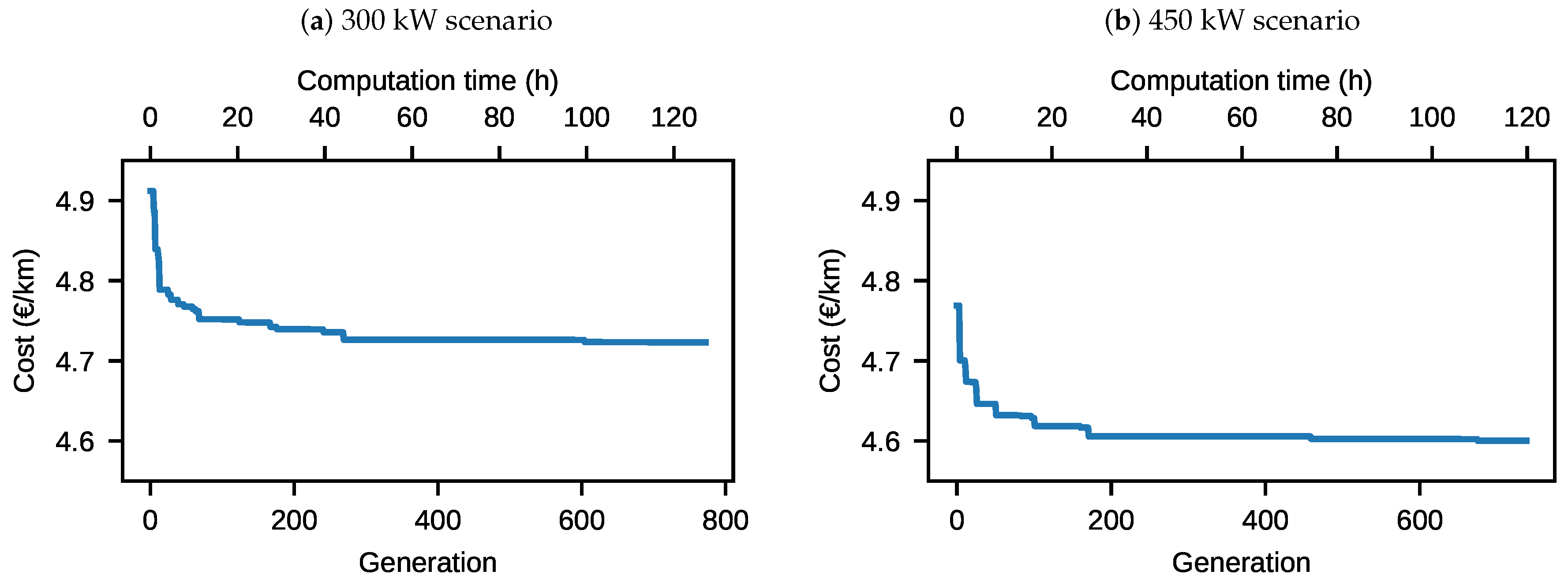
4.4. Genetic Algorithm for Charging Infrastructure Optimisation

The functions of eFLIPS presented thus far—electric bus scheduling, schedule simulation, year simulation and TCO calculation—require the specification of charging infrastructure locations as an input parameter. In the case of depot charging, this is trivial. When dealing with opportunity charging, however, deciding upon the location of charging points can become a complex task: As any combination of charging points poses a separate scheduling problem, the effect of charging point positions on overall system cost is difficult if not impossible to predict by intuition. Also, real-world bus networks produce solution spaces of considerable magnitude, as our case study presented in Section 5 will illustrate. It therefore seems purposeful to develop an optimisation method to determine a cost-optimised set of charging locations for opportunity charging.

To enable this, the entire process shown in Figure 3 was wrapped into a single function that returns the TCO of an electric bus system, using timetable data and charging point locations as the main inputs. A binary genetic algorithm (GA) was implemented that uses this aggregated TCO function as a fitness function.

A list of possible locations for OC charging infrastructure $L=(l_1,\dots ,l_i,\dots ,l_{N_{\mathrm{loc}}})$ defines the length $N_{\mathrm{loc}}$ of each chromosome $c=(b_1,\dots ,b_i,\dots ,b_{N_{\mathrm{loc}}})$. The position i of each allele maps to location $l_i$ and the value of the allele indicates whether a charging station is present at this location ($b_i=1$) or not ($b_i=0$). A population size $N_{\mathrm{pop}}$ is defined and an initial population is generated randomly. For each new generation, the best $N_{\mathrm{keep}}=x_{\mathrm{select}}{N}_{\mathrm{pop}}$ chromosomes are kept, $x_{\mathrm{select}}$ being the selection share, and the rest is discarded. Chromosome pairs (parents) are randomly selected to produce offspring through single-point crossover until the original population size is reached. The offspring is then mutated using the mutation rate $\mu$. We define $\mu$ as the share of alleles that is randomly modified, i.e., $N_{\mathrm{mut}}=⌈(N_{\mathrm{chrom}}-1)N_{\mathrm{loc}}\mu ⌉$ alleles at random positions are switched, $N_{\mathrm{chrom}}$ being the number of chromosomes in the population subset that mutation is applied to.

The number of charging slots is set to an arbitrary, high value for all stations in the schedule simulation so that, effectively, no capacity constraints exist. This is because the scheduling algorithm currently does not support charging station capacity constraints.

To reduce computation time, a simplified TCO calculation method was adopted for the GA fitness function: Instead of performing a year simulation using a temperature distribution, annual energy consumption is obtained by simply multiplying energy consumption for the critical consumption case by 365. Also, a static costing model is used.

Further reduction in computation time is obtained by skip** the fitness evaluation of infeasible solutions: Solutions not including at least one charging location per bus line are penalised by being assigned a very low fitness (i.e., high cost) value. Their actual TCO is not evaluated. Also, the algorithm caches all chromosomes and their respective fitness values such that no chromosome is evaluated twice. Parallel processing support was realised using Python’s multiprocessing package.

5. Case Study: Electrification Scenarios for an Urban Bus Network

To illustrate the application of our methodology, we conducted a case study for a real-world bus network consisting of 39 lines, of which 28 operate at daytime, 2 provide 24-hour service and 9 are night lines. For these lines, the current diesel bus schedules—from which the timetables can be generated by discarding the empty trips—and delay data were made available by the bus operator.

5.1. Vehicle Specifications and Energy Consumption

For the schedule simulation and TCO calculation, it is paramount to obtain representative vehicle parameters and consumption values. Our approach outlined in the following is to define a set of vehicle parameters based on market data, and to determine specific consumption for standard driving cycles by longitudinal dynamics simulation. The specific consumption obtained in this manner is later used for the constant consumption model in the schedule simulation.

5.1.1. Parameterising the Longitudinal Dynamics Model

Detailed standard on-road test (SORT) [50] test data was available from a bus manufacturer for an 18 m articulated electric bus. The test yields specific vehicle consumption in kWh/km for a SORT 1, 2 and 3 cycle using a fixed payload. These experimentally determined consumption values were used to parameterise and validate the vehicle model presented in Appendix C.

The parameters $f_{\mathrm{r}}$, $c_{\mathrm{w}}$, $A_{\mathrm{front}}$ and $\lambda$ used in Equations (A25) and (A26) were obtained from the literature (

Table 3. Parameters used for longitudinal dynamics simulations.

Quantity	Symbol	Value	Source
Rolling resistance coefficient	$f_{\mathrm{r}}$	0.0075	[51]
Drag coefficient	$c_{\mathrm{w}}$	0.66	[34]
Frontal projection area	$A_{\mathrm{front}}$	8.8 m${}^2$	[34]
Rotational mass factor	$\lambda$	1.1	[5]

). The HVAC system power $P_{\mathrm{HVAC}}$ is zero because the HVAC system was switched off during the SORT test. This leaves the total drivetrain efficiency ${\eta }_{\mathrm{total}}$ in Equation (A23) and the power of the remaining auxiliaries $P_{\mathrm{aux},\mathrm{other}}$ in Equation (A2) unknown. They were determined by least-squares approximation such that

$$\sum _{i=1}^3{\left(e_{\mathrm{SORT},i,\mathrm{sim}}-e_{\mathrm{SORT},i,\exp }\right)}^2\to min,$$

(3)

where $i=1\dots 3$ corresponds to the respective SORT profile, $e_{\mathrm{SORT},i,\mathrm{sim}}$ is the specific consumption obtained from longitudinal dynamics simulation and $e_{\mathrm{SORT},i,\exp }$ is the experimentally determined specific consumption. The least-squares approximation yielded ${\eta }_{\mathrm{total}}=0.86$ and $P_{\mathrm{aux},\mathrm{other}}=5.40\mathrm{kW}$, both of which are plausible (e.g., by comparison with Sinhuber et al. [34]). Using these parameters, the SORT cycle energy consumption obtained through simulation was within 2% of the experimentally determined consumption, as

Table 4. Comparison of simulated and experimentally determined energy consumption for standard on-road test (SORT) cycles.

Profile	Spec. Consumption (kWh/km)		Relative Deviation
	Simulation	Experiment
SORT 1	1.62	1.63	−0.5 %
SORT 2	1.43	1.40	+1.7 %
SORT 3	1.36	1.37	−1.1 %

indicates. The parameters will thus be used henceforth.

5.1.2. Defining Vehicle Types for the Simulation

We defined five base types of electric buses: Three depot charging types with low (120 km), medium (200 km) and high (300 km) range, and two opportunity charging types with a range of 60 km and different charging powers (300 kW and 450 kW). For each base type, parameters for a standard 12 m bus and an articulated 18 m bus were defined, yielding 10 electric bus configurations in total.

For each vehicle configuration, the battery capacity was set such that the desired range can be fulfilled on a SORT 2 cycle with 50% occupation on a very cold winter day (−10 °C) with the HVAC system enabled. Cabin temperature was set to 17 °C in accordance with the VDV guidelines on passenger cabin air-conditioning [52]. To ascertain that the range requirement can be satisfied even at the end of the battery lifetime, a battery state of health (SOH) of 80% was assumed. A root finder was used to obtain the matching battery capacity because the discrete-event simulation model does not permit solving for the battery capacity explicitly. The resulting battery weight was determined using energy density values taken from current manufacturer datasheets; for the high-range depot chargers, a 20% increase in energy density was assumed. Lithium-ion NMC batteries were assumed for the depot chargers and LTO batteries for the opportunity chargers. Vehicle base weights (without battery) were obtained as mean values from the literature. The full set of vehicle parameters used henceforth is listed in

Table 5. Vehicle parameters used for schedule simulation. Values of the form X/Y denote standard and articulated buses, respectively.

	Depot Charging			Opportunity Charging		Sources and Comments
	Short Range	Medium Range	Long Range	Low Power	High Power
Desired range (km)	120	200	300	60
Base weight (kg)	11175/16097					[53,54,55]
Kerb weight (kg)	12646/18164	13696/19638	14383/20604	13764/19734		Vehicle + battery
Maximum passenger occupation	70/99					[56]
UA value (kW/K)	0.562/0.843					Calculated from [57]
Insolation area (m${}^2$)	11.4/17.1
Aux power excl. HVAC (kW)	4.0/5.4					Simulation
Number of HVAC units	1/2
Battery parameters
- Energy density (Wh/kg)	171	171	205	53		[58,59]
- Capacity (kWh)	252/353	431/606	658/925	137/193		Simulation
- SOC (min-max)	0.05–0.95			0.10–0.95
- Maximum C rate	0.62			4.35		[58,59]
- SOH	0.80
Fast charging parameters
- Charging power (kW)				300	450
- Efficiency				0.95
- Dead time before-after (s)				15–15
Depot charging parameters
- Charging power (kW)	60–150
- Efficiency	0.95
- Dead time before-after (s)	60–60
Traction consumption (kWh/km) ${}^a$	0.73/0.99	0.77/1.05	0.80/1.09	0.77/1.06		Simulation
Total consumption (kWh/km) ${}^a$	1.51/2.12	1.55/2.18	1.58/2.22	1.55/2.18		Simulation

${}^a$ SORT 2, −10/17 °C, 50% occupation.

.

5.2. Simulation of Existing Schedules With Electric Buses

To assess the operability of the existing diesel bus schedules with electric buses, we performed simulations of the 317 unchanged schedules that cover the 39 lines on a weekday. Five scenarios, each corresponding to one of the vehicle types in Table 5, were simulated. Critical consumption parameters (SORT 2, 50% occupation, −10 °C outside, 17 °C inside) were assumed as outlined in the previous section.

For the opportunity charging scenarios, the location of charging stations has to be defined. (The word charging station is used synonymously with charging point; a station has several charging slots.) The charging optimisation algorithm introduced in Section 4.4 cannot be applied in this case because it enforces rescheduling of the vehicles. To avoid subjective decisions, a simple heuristic was chosen: A charging point was assumed at every terminus, even at termini that are only seldom visited. This yielded a total of 128 OC charging stations (more than three stations per line). It must be noted that this approach does not in any way reflect operational practice; it simply constitutes the upper boundary in terms of available energy supply and thus can be considered a theoretical best-case scenario for OC.

For the simulation of existing schedules, the question of interest is whether vehicles can sustain a valid state of charge during scheduled operation. Depot operations are irrelevant at this stage. Thus, no depot simulation was carried out; a new, fully charged vehicle was generated for each schedule. If vehicles arrived at a terminus delayed, the dwell time (and, therefore, the charging time in the OC cases) was shortened to permit a punctual departure whenever possible.

Simulation was carried out for punctual and delayed operation. For the latter case, historical delay data was available from the bus operator; the delay assigned to each trip was obtained as the 90th percentile of all delays observed on similar trips within the same hour of the day (similar trips are defined as trips on the same line in the same direction).

The simulation results are shown in Figure 9. It is observed that delays exert only a minor influence in the depot charging scenarios; in the opportunity charging scenarios, however, the results change considerably when delays are taken into account. As expected, the higher the DC vehicles’ range and the higher the OC vehicles’ charging power, the more schedules can be served. There is, however, no scenario that permits electric bus operation with completely unchanged schedules. Also, it must be emphasised that the OC results for a more realistic charging infrastructure setup would be considerably worse. These results reinforce our point that the transition to electric buses in a metropolitan bus network requires a rescheduling of vehicle operations [6].

5.3. Fully Electrified Scenarios: Scheduling and Charging Infrastructure Optimisation

We will now proceed to construct scenarios for fully electric bus operation. Six scenarios were generated: Five electric bus scenarios corresponding to the vehicle types in Table 5 and a diesel reference scenario for comparison. Diesel vehicles were modelled using a specific average consumption of 44.4 litres/100 km for standard buses and 59.4 litres/100 km for articulated buses (values from a bus operator’s fleet consumption evaluation over an entire year). HVAC system and other auxiliaries were not modelled for diesel buses, they were included in the average consumption.

For each of the scenarios, a new set of schedules has to be generated. In order to invoke the scheduling algorithm presented in Section 4.1, we first have to define a timetable. This is achieved by filtering the existing schedules for passenger trips on the specified lines. For the daytime lines, all trips during a weekday were chosen (this typically includes all trips between 4:00 a.m. and 1:00 a.m. of the following day). For the night lines, all trips departing on the evening of the same weekday and during the following night were considered. For the 24-hour lines, a time window must be chosen. We considered all trips departing between 3:00 a.m. and 2:59 a.m. on the following day, in accordance with the bus operator’s definition of an operational day. The resulting timetable consists of 4748 trips. All trips shall be served by a single depot.

For scheduling, the minimum dwell time was set to zero as some lines currently operate with zero dwell time at certain termini. Maximum dwell time and maximum deadheading time were set to 45 minutes. The average velocity used to compute the duration of deadhead trips was defined as 25 km/h. Line changes were only permitted during the second stage of scheduling (cf. Section 4.1). A reserve range of 10 km was assumed for all vehicle types and the effective battery capacity available for scheduling was reduced accordingly.

Delays were taken into account in all scenarios during scheduling: The minimum dwell time at every terminus was increased by the delay upon arrival such that a punctual departure for the succeeding trip is always possible. Technically, it would also be conceivable to consider delays only in the case of OC, since only OC requires “guaranteed” dwell times for recharging even in the presence of delays. However, this would imply the OC systems can maintain a higher level of punctuality than the DC and diesel systems. To ensure a consistent quality of service for the passenger in all scenarios, it is thus appropriate to always consider delays.

A cost-optimised charging station layout was determined for each of the OC scenarios using the genetic algorithm presented in Section 4.4. The parameters were: population size $N_{\mathrm{pop}}=120$, selection share $x_{\mathrm{select}}=0.5$ and mutation rate $\mu =0.2$. Infeasible solutions not including at least one charging station per bus line were assigned a TCO of 10 €/km. All of the 93 terminal stops were provided as charging location candidates, enabling $2^{93}\approx {10}^{28}$ possible combinations. Iteration was halted after approximately 5 days and 750 generations, having produced only incremental improvements once the infeasible solutions with a high cost penalty were removed from the population. A 12-core Intel Xeon E5-2640 machine with 64 GB RAM was used. Figure 10 shows the TCO of the best solution per generation over the course of the iteration. (Note that because of the simplified TCO model implemented within the GA, the TCO obtained by the GA does not match the TCO calculated in Section 5.5 using the full model.)

The genetic iteration yielded a set of 42 charging locations for the 300 kW scenario and 44 charging locations for the 450 kW scenario. These configurations were subsequently used for schedule generation and system simulation. Further discussion of the charging network optimisation results is found in Section 6.

The results of the scheduling process are listed in

Table 6. Scheduling statistics.

Case	Number of Schedules	Mean Distance (km)	Mean Duration (h)	Mean Efficiency (%)
DC (120 km)	667	96.7	5.9	88.2
DC (200 km)	441	138.6	8.6	91.5
DC (300 km)	350	171.2	10.7	92.8
OC (300 kW)	340	176.1	12.3	93.3
OC (450 kW)	327	182.3	12.4	93.4
Diesel	302	195.8	12.3	93.7

. The scheduling efficiency was determined for each schedule as the ratio

$${\eta }_{\mathrm{schedule}}=\frac{t_{\mathrm{productive}}}{t_{\mathrm{total}}},$$

(4)

where $t_{\mathrm{productive}}$ is the time spent during revenue service, i.e., on passenger trips excluding pauses, and $t_{\mathrm{total}}$ is the total operation time. Computing time for schedule generation was 333 s, or ≈56 s per scenario, on an Intel Core i5-6200U using a single core.

As would be expected, in the case of DC, the lower the vehicle range, the more schedules were generated and the lower is the resulting schedule efficiency. This is because more depot trips are required for the same number of passenger trips. The OC schedules provide higher efficiency than the DC schedules, indicating that the unproductive time for recharging OC vehicles is lower than the unproductive time for additional depot trips in the DC case. Diesel schedules have the highest mean efficiency and distance.

5.4. Fully Electrified Scenarios: System Simulation

The schedules generated for each technology in the previous section serve as the main input for the system simulation. The goal of the system simulation is to obtain the number of vehicles and charging points required to operate the schedules under critical conditions (a cold winter day as outlined in Section 5.2). Each individual vehicle is simulated; example SOC plots from a single-day simulation are given in Figure 11.

Schedules were generated for five electric bus scenarios (scenarios 1–5) and a diesel reference scenario (scenario 8) as illustrated in the previous section. Two additional electric bus scenarios (scenarios 6 and 7) not requiring additional scheduling were simulated to observe the impact of reducing the charging power at the depot: the medium range DC scenario and the low power OC scenario are replicated with a depot charging power of 60 kW instead of 150 kW.

To correctly simulate depot operations, the schedules have to be repeated twice such that a period of three consecutive days is simulated as illustrated in Figure 12: only on the second day will there exist an equilibrium state that reflects actual weekday depot operation. This is because at the beginning of the simulation, the depot starts empty and it takes some time until all vehicle objects have been generated; at the end of the simulation, all schedules have ended and all vehicles are returned to the depot. In reality, this never happens because a certain number of vehicles is always in service at any time of day.

The number of required fast charging slots was obtained as the sum of the maximum occupation of each charging station; an example is provided in Figure 13. The number of available slots per station was set to a high value in the simulation so that, effectively, charging station capacity was unconstrained. Vehicles were configured to occupy their charging slot until departure (see the discussion of queueing strategies in Section 4.2.2). The required number of depot charging slots was determined from the maximum depot occupation as illustrated in Figure 12. One depot charging slot per vehicle was assumed.

The simulation results are presented in

Table 7. Simulation results for fully electric scenarios and diesel reference scenario.

Scenario No.	Name	Fleet Size ${}^{\mathit{a}}$	Fast Charging Slots	Depot Charging Slots
1	DC (120 km)	116/188/304	0	272
2	DC (200 km)	130/206/336	0	305
3	DC (300 km)	94/143/237	0	205
4	OC (300 kW)	104/158/262	127	223
5	OC (450 kW)	100/154/254	117	215
6	DC (200 km), 60 kW	133/217/350	0	319
7	OC (300 kW), 60 kW	105/159/264	127	225
8	Diesel	94/140/234	0	201

${}^a$ Standard buses/articulated buses/total.

. We observe the following:

• Generally, the electric bus scenarios require at least 20 more vehicles (+12%) compared to the 234 vehicles in the diesel reference scenario. The only exception is the long-range DC scenario (scenario 3) that requires only three more vehicles (+1.3%).
• Reducing the charging power at the depot from 150 to 60 kW incurs a significantly larger fleet in the case of depot charging (+14 vehicles or 4%). In the case of opportunity charging, the increase in fleet size is less pronounced (+2 vehicles or 0.8%).
• Increasing the DC vehicles’ range from 120 to 200 km increases the required fleet size substantially by 32 vehicles or 10%. This is because in the 200 km case, many vehicles run out of energy during the afternoon when vehicle demand is at its peak and, thus, many new vehicles have to be generated. In the 120 km case, however, most vehicles return to the depot for charging before the afternoon peak and can then cover the entire afternoon shift uninterrupted. This surprising result illustrates the limits of the greedy scheduling algorithm: the objective pursued by the algorithm to maximise schedule length does not necessarily lead to a minimum fleet size.

5.5. Fully Electrified Scenarios: TCO Comparison

For the final step of our analysis, the TCO comparison, a year simulation was carried out for each of the scenarios to obtain annual energy demand and driver hours (see Section 4.3). A temperature function for Germany [60] was used and discretised into monthly intervals. Vehicle and infrastructure demand was taken from the simulation of the critical consumption case in the previous section. The cost parameters used in the TCO calculation are presented in

Table 8. TCO parameters. Values of the form X/Y denote standard and articulated buses, respectively.

Quantity	Value	Source
Base year and project start	2020	Assumption
Project duration	12 years	Assumption
Discount rate (general inflation)	1.4% p.a.	[61] (1999–2019)
Interest rate	4%	Assumption
Electric bus base cost (without battery)	450,000 €/585,000 €	Calculated based on [62,63,64] ${}^a$
Diesel bus cost	250,000 €/325,000 €	[62,63]
Vehicle lifetime	12 years	Assumption
Battery cost (NMC)	500 €/kWh	[64]
Battery cost (LTO)	800 €/kWh	Assumption
Battery cost escalation	−8% p.a.	Calculated based on [64]
Battery lifetime	6 years, 12 years	Assumption
300 kW fast charging station	200,000 € per slot	Own market research
450 kW fast charging station	250,000 € per slot	Own market research
Fast charging station construction/grid connection	225,000 € per station	Own market research
Depot charging station	100,000 € per slot	Own market research
Charging infrastructure lifetime	20 years	Assumption
Charging station efficiency	95%	Assumption
Electricity cost	0.15 €/kWh
Electricity cost escalation	+3.8% p.a.	[65] (2005–2019)
Diesel cost	1 €/L
Diesel cost escalation	+0.7% p.a.	[65] (2005–2019)
Fast charging station maintenance	1000 €/a per slot	Own market research

${}^a$ Price of standard electric bus [62]: 600 k€. Assuming a 300 kWh NMC battery, this leads to 450 k€ for the base bus. The articulated bus base cost was calculated assuming the same cost ratio as for diesel buses [62,63]: $450\mathrm{k}€·(325\mathrm{k}€/250\mathrm{k}€)=585\mathrm{k}€$.

. To obtain the driver hours, it was assumed that drivers are paid an additional 20 minutes per schedule for vehicle preparation and parking. Dwell times were only deducted from the paid labour hours if they have a certain minimum duration; short dwell times were assumed to be fully paid. This reflects the labour agreement of a bus operator, the details of which we cannot disclose. The cost for depot construction and depot grid connection was not considered. Identical unit cost was assumed for 150 and 60 kW depot charging points due to a lack of data. The construction and grid connection cost for fast charging stations was assumed equal for all stations, regardless of charging power and number of slots.

The eight scenarios were evaluated in two variants: One assuming a battery change after half of the bus lifetime, and the other without battery change. The results for both variants are shown in Figure 14. Vehicles and batteries are always treated as separate cost entities in the figures.

The key findings in the TCO comparison are:

• In the calculation with battery renewal, the lowest-cost DC electric bus scenario has a TCO 4–6% higher than the OC scenarios. Without battery renewal, this gap reduces to 1–2%.
• Reducing the depot charging power from 150 to 60 kW has a more pronounced impact on the TCO of the DC scenario (+2%) than on the TCO of the OC scenario (+0.2%), as would be expected from the vehicle demand presented in the previous section.
• If no battery renewal is necessary, system cost is reduced by 2% to 4%.
• The short-range and long-range DC scenarios have equal TCO if battery renewal is considered; in this case, the reduced vehicle demand in the long-range scenario is countered by higher battery replacement cost. The calculation without battery renewal, however, favours the long-range scenario, albeit by a narrow margin (−2.5% compared to the short-range scenario).
• The 450 kW OC scenario is slightly more competitive than the 300 kW scenario by a very small margin (−1%).
• Charging infrastructure has little influence on TCO: Its contribution ranges from 0.6% to 1.0% for DC and from 3.0% to 3.4% for OC.
• Staff cost (driver wages) accounts for 50% to 64% of TCO depending on the scenario. The electric bus scenarios increase the staff cost by the following, compared to the diesel scenario: DC (120 km): 8%; DC (200 km): 3%; DC (300 km): 1%; OC (300 kW): 5%; OC (450 kW): 4%.
• The electric bus scenarios incur an overall TCO 15–31% higher than the diesel scenario if battery renewal is considered, and 13–25% without battery renewal.

6. Discussion

In this section, we will address the limitations of our methodology and critically evaluate our results.

6.1. OC Infrastructure Optimisation

The result obtained by the charging infrastructure optimisation−42 stations in the 300 kW scenario and 44 in the 450 kW scenario—appears counterintuitive at first. It would be expected that the lower the charging power, the more charging stations have to be deployed. However, our result can be explained by the behaviour of the scheduling algorithm: Dwell times are determined such that the battery can be fully charged at every terminus with a charging facility. Due to this strict condition, a lower charging power increases the chance of the algorithm skip** the next departure at a terminus, as illustrated schematically in Figure 15. If departures are skipped, however, the dwell time increases by a multiple of the headway—creating additional time available for charging. This can eliminate the need for additional charging stations on the same line. A high charging power, on the other hand, increases the chance of obtaining a full charge without skip** departures, thus requiring more charging stations, but reducing vehicle demand.

In practice, it would be conceivable to adjust timetables in order to better accommodate opportunity charging and further reduce charging infrastructure demand. For example, departure times could be modified such that the resulting dwell times are shifted toward one terminus, thus allowing operation of the respective line with only one charging station. However, this was outside of the scope of this study.

6.2. Scheduling

As illustrated in Section 5.4, the greedy scheduling algorithm does not construct schedules with minimum vehicle demand, which can lead to unexpected results especially in the case of DC. The algorithm is therefore of limited use for schedule planning in practical applications. Optimisation-based approaches as introduced in Section 3.2 are better suited, but issues regarding the implementation and the ability to solve large problem instances have to be considered. In the case of OC, the algorithm cannot consider charging station capacity constraints. This also is an obstacle to practical application as the physical space available at potential charging locations is usually limited from the outset.

6.3. Vehicle and Infrastructure Demand (System Simulation)

The OC charging infrastructure demand determined in the simulation is comparatively high in relation to the fleet size: In both OC scenarios (4 and 5), it amounts to one charging slot for every two vehicles. This figure could be lowered significantly in two ways. Firstly, charging slots that are only seldom occupied could be dispensed of. Figure 13 provides an example: The peak demand of eight slots only occurs three times a day for short intervals. Because vehicles generally have an ample SOC reserve in the simulation, eliminating the eighth charging slot should have no adverse effects (but this would have to be confirmed by a separate simulation). Secondly, changing the queueing strategy at charging stations could enable a major reduction in charging points: In an unpublished study we conducted for a bus operator, enabling vehicles to release charging points once fully charged reduced the number of required charging points by 17%. However, this may incur additional staff cost, depending on the labour regulations. Generally, the effect of reducing the number of charging slots on overall TCO is expected to be marginal as charging infrastructure contributes no more than 3.4% to the TCO.

6.4. TCO calculation

Our TCO results presented in Section 5.5 are not directly comparable to values from the literature because the majority of works does not consider staff cost (as outlined in Section 3.5). For better comparability, Figure 16 shows the results including only the additional staff cost incurred by electric bus operation compared to the diesel scenario (i.e., the staff cost in the diesel scenario is set to zero). Because of the infeasible scheduling results, the medium-range DC scenarios were omitted.

Table 9. Comparison of TCO results from the literature.

Source	Relative TCO Difference			Comments
	OC vs. Diesel	DC vs. Diesel	DC vs. OC
Bi et al. [13]	−18%	−12%	8%	No staff cost
Kunith [5]	4 … 18%	53 … 83%	47 … 55%	Additional staff cost (for DC only)
Lajunen and Lipman [11]	22 … 29%	34 … 44%	7 … 18%	No staff cost
Pihlatie et al. [26]	7 … 25%	43 … 60%	26 … 40%	No staff cost
Vilppo and Markkula [21]	−6%	n/a	n/a	No staff cost
Ke et al. [16]	n/a	n/a	8%	No staff cost
This work	35 … 45%	42 … 58%	6 … 13%	Additional staff cost

shows the relative TCO differences between individual technologies (diesel, OC, DC) determined from the literature as well as our results from Figure 16. There are considerable discrepancies between the values. Some studies claim a cost advantage of electric over diesel buses at recent prices; our findings disagree with this. Furthermore, some studies estimate a high cost difference between DC and OC of up to 55%, which we also cannot confirm. This is due to the fact that none of the studies consider the additional staff cost incurred by OC and that some studies assume charging at intermediate stops (as outlined in Section 3.5), reducing the cost of the OC system. The results by Lajunen and Lipman [11] are closest to ours, but even here, considerable deviations remain due to methodological differences.

The cost for modifications to the bus depot was not considered in our study. It is expected to be higher for DC than for OC because of the larger fleet size and more powerful grid connection required. Thus, the cost gap between the two technologies could widen when considering depot construction. On the other hand, the planning and operation of OC charging infrastructure on public roads may also incur additional cost not considered in our model.

In light of the narrow cost difference observed between some scenarios, it must be noted that cost parameters may be subject to high uncertainties. In particular, the cost of vehicles and charging infrastructure is difficult to determine due to the scarcity of public data and the highly individualised nature of bus procurements. Also, there seem to be large cost differences between various manufacturers as vehicle prices determined from the literature show (Figure 17): Cost differences of up to one-third are observed despite similar battery capacity.

7. Conclusions and Outlook

We developed a planning and simulation methodology for electric bus networks comprising an object-oriented, discrete-event based simulation tool, a greedy bus scheduling algorithm, and a genetic algorithm for charging infrastructure positioning wrapped around the scheduling algorithm and simulation. The methodology was applied to assess the electrification of a real-world, metropolitan bus network with 39 bus lines using depot charging (DC) and opportunity charging at terminal stops (OC-T).

We first investigated the feasibility of operating existing diesel bus schedules with electric buses. Five electric bus scenarios were evaluated: three DC scenarios with varying range (120, 200 and 300 km) and two OC scenarios with varying charging power (300 and 450 kW). The analysis shows that none of the scenarios permit the operation of unchanged schedules, owing to the limited range of DC buses and the limited charging time available for OC. Delays exert a significant influence in the OC case and must therefore be taken into account to obtain valid results.

In the second stage, a TCO evaluation was carried out for fully electrified scenarios and a diesel reference scenario. New schedules were planned for each scenario using our scheduling algorithm. For OC, TCO-optimised charging locations were obtained using the genetic algorithm. We found that the smallest electric bus fleet size could be achieved by DC buses with a range of 300 km; otherwise, the OC scenarios yielded smaller fleet sizes than DC. The charging process at the depot was identified as a bottleneck for DC, but not for OC buses.

The TCO calculation reveals that OC has a slight cost advantage over DC in all scenarios, the TCO of DC being 1–6% higher than OC. As depot construction cost was not considered, the cost gap between DC and OC may turn out higher in practice. Compared to diesel systems, the TCO of OC was at least 13% higher and the TCO of DC was at least 15% higher. Contrary to other studies, these figures include the full driver cost, allowing an assessment of the true additional cost of electric bus operation on a system level.

Our analysis of a complete bus network confirms our previous finding for a single bus line in [6]: On a system level, the cost difference between OC and DC can turn out very small. Given the uncertainties of the inputs, it can be argued that de facto cost parity exists between the two systems under some circumstances. Thus, no general recommendation for either of the technologies can be given solely on a cost basis. In cases where the results of the TCO analysis are inconclusive, other criteria must be defined to decide upon one of the two technologies.

Our methodology provides a framework for the planning and evaluation of electric bus systems with a higher level of detail and less reliance on simplifying assumptions than approaches found in the existing literature. Nonetheless, several aspects could be improved in further research:

• The strict condition to fully charge at every charging station enforced by the scheduling algorithm reduces the efficiency of the OC schedules.
• The objective of the scheduling algorithm—maximising the schedule length—does not concur with the objective of minimum fleet size or minimum cost, leading to partly unexpected results especially in the case of DC. Development of a refined algorithm is already underway. It takes into account the concurrence of trips and leads to a more even distribution of depot trips over time, potentially mitigating the adverse effect observed in this work.
• The scheduling algorithm currently does not support charging station capacity constraints.
• In this study, we limited the duration of an operational day to 24 h. However, with OC, vehicles could remain in service for several consecutive days without returning to the depot, reducing the number of depot trips and, therefore, the TCO. This should be examined in future works.
• We did not evaluate a mixed scenario of OC and DC lines, even though it is a likely option for real-world application. Determining the best choice of technology on a per-line basis is, however, an optimisation problem in itself, requiring the development of additional methodology.
• The possibility of opportunity charging with central charging stations (OC-C) was not evaluated. This would also require further development of the scheduling algorithm.
• The schedule simulation currently relies on a simple, constant consumption vehicle model. This should be improved especially if the topography of the bus network includes steep gradients.
• The battery model currently does not consider variable charging power depending on the current state of charge. Also, no evaluation of the battery lifetime based on the actual charging/discharging cycle (e.g., as in [68]) is carried out. Both could be improved for better accuracy.

References

1. ZeEUS Project. ZeEUS eBus Report #2: An Updated Overview of Electric Buses in Europe. Available online: http://zeeus.eu/uploads/publications/documents/zeeus-report2017-2018-final.pdf (accessed on 25 June 2020).
2. Verband deutscher Verkehrsunternehmen (VDV). E-Bus-Projekte in Deutschland. Available online: https://www.vdv.de/e-bus-projekt.aspx (accessed on 25 June 2020).
3. Wilkens, A. Induktives Laden: Mannheim Will Keine Weiteren Primove-Elektrobusse. Available online: https://www.heise.de/newsticker/meldung/Induktives-Laden-Mannheim-will-keine-weiteren-Primove-Elektrobusse-4060084.html (accessed on 25 June 2020).
4. Sommariva, R. Trolleybuses in Berlin, BVG is Considering Massive Deployment in Spandau District. Available online: https://www.sustainable-bus.com/news/trolleybuses-in-berlin-bvg-is-considering-massive-deployment-in-spandau-district/ (accessed on 25 June 2020).
5. Kunith, A.W. Elektrifizierung des Urbanen öffentlichen Busverkehrs: Technologiebewertung für den Kosteneffizienten Betrieb Emissionsfreier Bussysteme. Ph.D. Thesis, Technische Universität Berlin, Berlin, Germany, 2017. [Google Scholar] [CrossRef]
6. Jefferies, D.; Göhlich, D. Integrated TCO Assessment of Bus Network Electrification Considering Rescheduling and Delays: Modelling Framework and Case Study. EVS31 International Electric Vehicle Symposium & Exhibition, Kobe, Japan. 2018. Available online: https://www.researchgate.net/publication/329210166_Integrated_TCO_Assessment_of_Bus_Network_Electrification_Considering_Rescheduling_and_Delays (accessed on 25 June 2020).
7. Göhlich, D.; Fay, T.A.; Jefferies, D.; Lauth, E.; Kunith, A.; Zhang, X. Design of urban electric bus systems. Des. Sci. 2018, 4. [Google Scholar] [CrossRef] [Green Version]
8. Fusco, G.; Alessandrini, A.; Colombaroni, C.; Valentini, M.P. A Model for Transit Design with Choice of Electric Charging System. Procedia-Soc. Behav. Sci. 2013, 87, 234–249. [Google Scholar] [CrossRef] [Green Version]
9. Lajunen, A. Lifecycle costs and charging requirements of electric buses with different charging methods. J. Clean. Prod. 2018, 172, 56–67. [Google Scholar] [CrossRef]
10. Gao, Z.; Lin, Z.; LaClair, T.J.; Liu, C.; Li, J.M.; Birky, A.K.; Ward, J. Battery capacity and recharging needs for electric buses in city transit service. Energy 2017, 122, 588–600. [Google Scholar] [CrossRef] [Green Version]
11. Lajunen, A.; Lipman, T. Lifecycle cost assessment and carbon dioxide emissions of diesel, natural gas, hybrid electric, fuel cell hybrid and electric transit buses. Energy 2016, 106, 329–342. [Google Scholar] [CrossRef]
12. Macedo, J.; Soares, G.; Kokkinogenis, Z.; Perrotta, D.; Rossetti, R.J.F. A Framework for Electric Bus Powertrain Simulation in Urban Mobility Settings: Coupling SUMO with a Matlab/Simulink Nanoscopic Model, 1st ed.; SUMO User Conference: Berlin, Germany, 2013. [Google Scholar]
13. Bi, Z.; de Kleine, R.; Keoleian, G.A. Integrated Life Cycle Assessment and Life Cycle Cost Model for Comparing Plug-in versus Wireless Charging for an Electric Bus System. J. Ind. Ecol. 2017, 21, 344–355. [Google Scholar] [CrossRef]
14. De Filippo, G.; Marano, V.; Sioshansi, R. Simulation of an electric transportation system at The Ohio State University. Appl. Energy 2014, 113, 1686–1691. [Google Scholar] [CrossRef]
15. Sebastiani, M.T.; Luders, R.; Fonseca, K.V.O. Evaluating Electric Bus Operation for a Real-World BRT Public Transportation Using Simulation Optimization. IEEE Trans. Intell. Transp. Syst. 2016, 17, 2777–2786. [Google Scholar] [CrossRef]
16. Ke, B.R.; Chung, C.Y.; Chen, Y.C. Minimizing the costs of constructing an all plug-in electric bus transportation system: A case study in Penghu. Appl. Energy 2016, 177, 649–660. [Google Scholar] [CrossRef]
17. Rogge, M.; van der Hurk, E.; Larsen, A.; Sauer, D.U. Electric bus fleet size and mix problem with optimization of charging infrastructure. Appl. Energy 2018, 211, 282–295. [Google Scholar] [CrossRef] [Green Version]
18. Lindgren, L. Electrification of City Bus Traffic-A Simulation Study Based on Data from Linkö**. Available online: http://lup.lub.lu.se/record/d5834bb3-c0f0-4c7c-a493-69b10291d1f1 (accessed on 25 June 2020).
19. Li, L.; Lo, H.K.; **ao, F. Mixed bus fleet scheduling under range and refueling constraints. Transp. Res. Part Emerg. Technol. 2019, 104, 443–462. [Google Scholar] [CrossRef]
20. Kovalyov, M.Y.; Rozin, B.M.; Guschinsky, N.N. Mathematical Model and Random Search Algorithm for the Optimal Planning Problem of Replacing Traditional Public Transport with Electric. Autom. Remote Control. 2020, 81, 803–818. [Google Scholar] [CrossRef]
21. Vilppo, O.; Markkula, J. Feasibility of electric buses in public transport. In Proceedings of the EVS28 International Electric Vehicle Symposium and Exhibition, Seoul, Korea, 3–5 May 2015. [Google Scholar]
22. Kunith, A.; Mendelevitch, R.; Göhlich, D. Electrification of a city bus network-An optimization model for cost-effective placing of charging infrastructure and battery sizing of fast charging electric bus systems. DIW Discussion Papers. 2016. Available online: http://www.diw.de/documents/publikationen/73/diw_01.c.534056.de/dp1577.pdf (accessed on 25 June 2020).
23. Liu, Z.; Song, Z. Robust planning of dynamic wireless charging infrastructure for battery electric buses. Transp. Res. Part Emerg. Technol. 2017, 83, 77–103. [Google Scholar] [CrossRef]
24. Berthold, K.; Förster, P.; Rohrbeck, B. Location Planning of Charging Stations for Electric City Buses. In Operations Research Proceedings; Springer International Publishing: Cham, Switzerland, 2017; pp. 237–242. [Google Scholar] [CrossRef]
25. Xylia, M.; Leduc, S.; Patrizio, P.; Kraxner, F.; Silveira, S. Locating charging infrastructure for electric buses in Stockholm. Transp. Res. Part Emerg. Technol. 2017, 78, 183–200. [Google Scholar] [CrossRef]
26. Pihlatie, M.; Kukkonen, S.; Halmeaho, T.; Karvonen, V.; Nylund, N.O. Fully electric city buses-The viable option. In Proceedings of the 2014 IEEE International Electric Vehicle Conference (IEVC), Florence, Italy, 17–19 December 2014; pp. 1–8. [Google Scholar] [CrossRef]
27. Paul, T.; Yamada, H. Operation and charging scheduling of electric buses in a city bus route network. In Proceedings of the 17th International IEEE Conference on Intelligent Transportation Systems (ITSC), Qingdao, China, 8–11 October 2014. [Google Scholar] [CrossRef]
28. Wang, H.; Shen, J. Heuristic approaches for solving transit vehicle scheduling problem with route and fueling time constraints. Appl. Math. Comput. 2007, 190, 1237–1249. [Google Scholar] [CrossRef]
29. Li, J.Q. Transit Bus Scheduling with Limited Energy. Transp. Sci. 2014, 48, 521–539. [Google Scholar] [CrossRef]
30. Adler, J.D.; Mirchandani, P.B. The Vehicle Scheduling Problem for Fleets with Alternative-Fuel Vehicles. Transp. Sci. 2017, 51, 441–456. [Google Scholar] [CrossRef]
31. Wen, M.; Linde, E.; Ropke, S.; Mirchandani, P.; Larsen, A. An adaptive large neighborhood search heuristic for the Electric Vehicle Scheduling Problem. Comput. Oper. Res. 2016, 76, 73–83. [Google Scholar] [CrossRef] [Green Version]
32. Reuer, J.; Kliewer, N.; Wolbeck, L. The Electric Vehicle Scheduling Problem-A study on time-space network based and heuristic solution approaches. In Proceedings of the Conference on Advanced Systems in Public Transport (CASPT), Rotterdam, The Netherlands, 19–23 July 2015. [Google Scholar]
33. van Kooten Niekerk, M.E.; van den Akker, J.M.; Hoogeveen, J.A. Scheduling electric vehicles. Public Transp. 2017, 9, 155–176. [Google Scholar] [CrossRef]
34. Sinhuber, P.; Rohlfs, W.; Sauer, D.U. Study on Power and Energy Demand for Sizing the Energy Storage Systems for Electrified Local Public Transport Buses. In Proceedings of the IEEE Vehicle Power and Propulsion Conference (VPPC), Seoul, Korea, 9–12 October 2012; pp. 315–320. [Google Scholar]
35. Hegazy, O.; El Baghdadi, M.; Coosemans, T.; Van Mierlo, J. Co-design Optimization Framework for Electrified Buses in Cities:Brussels Case Study. In Proceedings of the EVS31 International Electric Vehicle Symposium & Exhibition, Kobe, Japan, 30 September–3 October 2018. [Google Scholar]
36. Lajunen, A.; Kalttonen, A. Investigation of thermal energy losses in the powertrain of an electric city bus. In Proceedings of the 2015 IEEE Transportation Electrification Conference and Expo (ITEC), Dearborn, Michigan, 14–17 June 2015. [Google Scholar] [CrossRef]
37. Jefferies, D.; Ly, T.; Kunith, A.; Göhlich, D. Energiebedarf Verschiedener Klimatisierungssysteme für Elektro-Linienbusse; Deutsche Kälte- und Klimatagung: Dresden, Germany, 2015. [Google Scholar]
38. Göhlich, D.; Ly, T.; Kunith, A.; Jefferies, D. Economic assessment of different air-conditioning and heating systems for electric city buses based on comprehensive energetic simulations. In Proceedings of the EVS28 International Electric Vehicle Symposium and Exhibition, Seoul, Korea, 3–5 May 2015. [Google Scholar]
39. Jäger, B.; Wittmann, M.; Lienkamp, M. Agent-based Modeling and Simulation of Electric Taxi Fleets. 6. Conference on Future Automotive Technology; Fürstenfeldbruck, Germany, 2017. Available online: https://mediatum.ub.tum.de/1378513 (accessed on 25 June 2020).
40. Gacias, B.; Meunier, F. Design and operation for an electric taxi fleet. OR Spectrum 2014, 37, 171–194. [Google Scholar] [CrossRef] [Green Version]
41. Cheng, S.F.; Nguyen, T.D. TaxiSim: A Multiagent Simulation Platform for Evaluating Taxi Fleet Operations. IEEE/WIC/ACM International Conference on Intelligent Agent Technology. 2011. Available online: https://works.bepress.com/sfcheng/1/ (accessed on 25 June 2020).
42. van Lon, R.R.S.; Holvoet, T. RinSim: A Simulator for Collective Adaptive Systems in Transportation and Logistics. In Proceedings of the 2012 IEEE Sixth International Conference on Self-Adaptive and Self-Organizing Systems, Lyon, France, 10–14 September 2012. [Google Scholar] [CrossRef] [Green Version]
43. Meignan, D.; Simonin, O.; Koukam, A. Simulation and evaluation of urban bus-networks using a multiagent approach. Simul. Model. Pract. Theory 2007, 15, 659–671. [Google Scholar] [CrossRef]
44. Cats, O.; Larijani, A.N.; Koutsopoulos, H.N.; Burghout, W. Impacts of Holding Control Strategies on Transit Performance. Transp. Res. Rec. J. Transp. Res. Board 2011, 2216, 51–58. [Google Scholar] [CrossRef] [Green Version]
45. Lajunen, A. Energy consumption and cost-benefit analysis of hybrid and electric city buses. Transp. Res. Part Emerg. Technol. 2014, 38, 1–15. [Google Scholar] [CrossRef]
46. Lauth, E.; Mundt, P.; Göhlich, D. Simulation-based Planning of Depots for Electric Bus Fleets Considering Operations and Charging Management. In Proceedings of the 4th International Conference on Intelligent Transportation Engineering (ICITE), Singapore, 7 September 2019. [Google Scholar] [CrossRef]
47. Python Software Foundation. Python. Available online: https://www.python.org/ (accessed on 25 June 2020).
48. Scherfke, S. SimPy: Discrete Event Simulation for Python. Available online: https://simpy.readthedocs.io/en/latest/ (accessed on 25 June 2020).
49. Heidelberg Institute for Geoinformation Technology (HeiGIT). Openrouteservice. Available online: https://openrouteservice.org/ (accessed on 25 June 2020).
50. UITP. UITP Project “SORT”–Standardised on-Road Test Cycles; UITP: Brussels, Belgium, 2009. [Google Scholar]
51. Mitschke, M.; Wallentowitz, H. Dynamik der Kraftfahrzeuge; Springer Fachmedien Wiesbaden: Wiesbaden, Germany, 2014. [Google Scholar] [CrossRef]
52. Verband Deutscher Verkehrsunternehmen (VDV). VDV-Schrift 236: Klimatisierung von Linienbussen der Zulassungsklassen I und II, Für Konventionell Angetriebene Diesel- und Gasbusse Sowie Für Hybrid-, Brennstoffzellen- und Elektrobusse; VDV: Cologne, Germany, 2015. [Google Scholar]
53. Bünnagel, C. Irizar ie bus-Power aus dem Baskenland. Verk. Tech. 2018, 10, 363–369. [Google Scholar] [CrossRef]
54. Ebusco. The New Ebusco 2.2. Available online: https://www.ebusco.com/wp-content/uploads/EBUSCO_brochure_2-2_digi.pdf (accessed on 25 June 2020).
55. Hondius, H. Daimler Buses stellt vollelektrischen Mercedes-Benz Citaro vor. Stadtverkehr 2018, 5, 10–15. [Google Scholar]
56. Berliner Verkehrsbetriebe AöR (BVG). Die Omnibusflotte der BVG. Available online: https://unternehmen.bvg.de/index.php?section=downloads&download=579 (accessed on 25 June 2020).
57. Färber, F. Heizen im Elektrobus. In Proceedings of the 10. VDV-Konferenz Elektrobusse, Berlin, Germany, 5–6 February 2019. [Google Scholar]
58. Akasol AG. Akasol Akasystem 15 AKM 64 CYC. Available online: https://www.akasol.com/library/Downloads/Datenbl%C3%A4tter/02-05-2019/Data%20sheet-AKASOL-AKASystem-15AKM64CYC-WEB.pdf (accessed on 25 June 2020).
59. Impact Clean Power Technology S.A. UVES LTO Standard Battery Pack LTO 15.2 kWh. Available online: https://icpt.pl/wp-content/uploads/2018/07/ICPT_UVES_LTO_Standard_leaflet.pdf (accessed on 25 June 2020).
60. Bundesinstitut für Bau-, Stadt- und Raumforschung. Aktualisierte und Erweitere Testreferenzjahre (TRY) von Deutschland für Mittlere und Extreme Witterungsverhältnisse. Available online: http://www.bbsr-energieeinsparung.de/EnEVPortal/DE/Regelungen/Testreferenzjahre/Testreferenzjahre/01_start.html?nn=739044&notFirst=true&docId=743442 (accessed on 25 June 2020).
61. Statistisches Bundesamt. Genesis-Online: Die Datenbank des Statistischen Bundesamtes. Available online: https://www-genesis.destatis.de/genesis/online (accessed on 25 June 2020).
62. Fülling, T. Neue Berliner E-Busse können nur halben Tag fahren. Available online: https://www.morgenpost.de/berlin/article226090187/Neue-E-Busse-in-Berlin-koennen-nur-halben-Tag-fahren.html (accessed on 25 June 2020).
63. Fülling, T. BVG kauft 156 neue Busse im “Schweden-Design”. Available online: https://www.morgenpost.de/berlin-aktuell/article122117680/BVG-kauft-156-neue-Busse-im-Schweden-Design.html (accessed on 14 July 2020).
64. Sauer, D.U. Aktueller Stand der Entwicklungen von Batterietechnik und Batteriemarkt. In Proceedings of the 11. VDV-Konferenz Elektrobusse, Berlin, Germany, 4–5 February 2020. [Google Scholar]
65. Statistisches Bundesamt. Daten zur Energiepreisentwicklung-Lange Reihen bis März 2020. Available online: https://www.destatis.de/DE/Themen/Wirtschaft/Preise/Publikationen/Energiepreise/energiepreisentwicklung-pdf-5619001.html (accessed on 25 June 2020).
66. Krämer, K.; Hanke, D. Lange Stille. Bozankaya Elektrobus Sileo S 12. Omnibusspiegel 2015, 2, 5–9. [Google Scholar]
67. Kölner Verkehrs-Betriebe AG. KVB stellt den Betrieb der Linie 133 auf E-Busse um: Zehnmonatiges Testprogramm wurde erfolgreich abgeschlossen: Pressemitteilung. Available online: https://www.presseportal.de/pm/122503/3501162 (accessed on 25 June 2020).
68. Göhlich, D.; Fay, T.A.; Park, S. Conceptual Design of Urban E-Bus Systems with Special Focus on Battery Technology. Proc. Des. Soc. Int. Conf. Eng. Des. 2019, 1, 2823–2832. [Google Scholar] [CrossRef] [Green Version]
69. Verein deutscher Ingenieure (VDI). VDI-Richtlinie 2078: Berechnung von Kühllast und Raumtemperaturen von Räumen und Gebäuden; VDI: Düsseldorf, Germany, 2012. [Google Scholar]
Figure 1. Electric bus charging strategies.
Wevj 11 00056 g001
Figure 2. Generalised workflow of electric bus system planning and TCO evaluation, including examples of methods and data commonly used in the literature.
Wevj 11 00056 g002
Figure 3. Overview of eFLIPS (Electric Fleet and Infrastructure Planning/Simulation) main features and workflow.
Wevj 11 00056 g003
Figure 4. Simplified overview of the relationships between objects in the schedule simulation.
Wevj 11 00056 g004
Figure 5. Vehicle and energy subsystem model.
Wevj 11 00056 g005
Figure 6. Actions controlled by charging logic.
Wevj 11 00056 g006
Figure 7. Vehicle demand calculation.
Wevj 11 00056 g007
Figure 8. TCO calculation method.
Wevj 11 00056 g008
Figure 9. Results from the simulation of existing diesel bus schedules with electric buses. The pie charts indicate the number of schedules for which the following applies: Green—schedules can be served within the state of charge (SOC) limits of the battery and also leave an operational safety margin of 10 km; yellow—schedules can technically be operated, but violate the 10 km safety margin; red—schedules are inoperable because they violate the SOC limits of the battery.
Wevj 11 00056 g009
Figure 10. Progress of charging infrastructure optimisation.
Wevj 11 00056 g010
Figure 11. Typical vehicle SOC time series from schedule simulation.
Wevj 11 00056 g011
Figure 12. Using repeated schedules to obtain an equilibrium state in the bus depot.
Wevj 11 00056 g012
Figure 13. Example of opportunity charging (OC) charging point occupation.
Wevj 11 00056 g013
Figure 14. TCO results for all scenarios. S: standard bus; A: articulated bus.
Wevj 11 00056 g014
Figure 15. Schematic illustration of the effect of charging power on charging station placement using the greedy scheduling algorithm.
Wevj 11 00056 g015
Figure 16. TCO comparison after subtracting staff cost of diesel scenario. S: standard bus; A: articulated bus.
Wevj 11 00056 g016
Figure 17. Comparison of vehicle cost reported in the literature [53,62,66,67].
Wevj 11 00056 g017